Machine Learning in Finance · Session 1
Machine Learning in Finance · Session 1
Programming and machine learning for people who have never written a line of code. We start from zero.
jobo@econ.au.dk, whoever is lecturing. Bezirgen Veliyev lectures some of the sessions.
Finance has become a data discipline.
The goal is not to make you a computer scientist. It is to let you read, build, and judge the models that finance now runs on.
Your OLS regression is already a simple machine-learning model: it learns its coefficients from data. We build outward from there.
Thirteen sessions, from the week of 31 August 2026 (week 36) to week 42.
Lectures are for watching and understanding. You learn to code by doing the exercises and the case yourself, between sessions.
Going from no programming to machine learning in seven weeks is a steep climb. Be ready for it.
My job is to teach the concepts and point the way. Your job is to do the work.
AI assistants are useful and are not banned. Use them to learn, not to avoid learning.
A good test: if you could not rewrite it from memory afterwards, you have not learned it yet.
The exam runs on your own machine, offline. We begin in Google Colab because it is the easiest place to start, and later move to a local setup: a VS Code tutorial comes in Session 3.
Because the exam is offline, the skill has to be yours. That is the whole reason the exercises matter.
By the end of this session you can:
And you meet the course case: a four-part risk report on real US stocks.
Part 1
Where our code lives, and how a code cell shows its result.
A notebook is a document read top to bottom, made of two kinds of cell. The result of a code cell appears directly beneath it.
That is the whole idea. A lecture, a calculation, and its result can live in one scrollable document, which is exactly what these slides are.
We begin in Google Colab, which runs notebooks in your browser with nothing to install. You need only a Google account.
Click into a code cell and press Ctrl + Enter. The cell runs and shows the value of its last line, and only the last one.
These slides run Python too. Run this: just one number appears.
A real Python cell, running in your browser. Change the numbers and run it again. Clicking Run does exactly the same thing.
| key | what it does | where |
|---|---|---|
Ctrl + Enter |
runs the cell, stays put | everywhere, including these slides |
Shift + Enter |
runs the cell, moves to the next | Colab, Jupyter, VS Code |
On a Mac, use Cmd in place of Ctrl.
Shift + Enter is the habit most people settle into in Colab. The little editor built into these slides is the one place it does nothing at all, so here use Ctrl + Enter or the Run button.
To show several values, use print(...):
print is our first function: a named tool you use by writing its name and round brackets. It displays whatever you put inside, each on its own line. We will lean on it constantly.
Part 2
Expressions, and leaving notes to yourself.
An expression is code that produces a value. The text after a # is a comment: Python ignores it; it is a note for humans.
Change the numbers and run it. Arithmetic works as you would expect.
| write | meaning |
|---|---|
+ - * / |
add, subtract, multiply, divide |
** |
power: 1.05 ** 10 is ten years of 5% growth |
( ) |
grouping, exactly as in mathematics |
Order of operations is the usual one: powers, then * and /, then + and -. Parentheses override it.
1,000 invested at 4% for five years is a single expression:
Change the rate to 0.06 and run again. Compounding is just repeated multiplication, written with **.
Part 3
Giving a value a name, so you can use it again.
A variable gives a value a name. The = sign means assign: “store this under that name”, not “equals”.
Anywhere you write the name, Python uses the value:
holding_value now holds the result, ready to reuse, with no need to retype the multiplication.
Assigning to a name that already exists replaces its value. The old one is gone.
Read price = price * 1.02 from the right:
take the current
price, multiply by 1.02, and store the result back intoprice.
Line 2 uses price on both sides at once. What do you think that does, and what is price at the end? Reason it out before you run.
Can a name really appear on both sides of =?
Python requires:
share price fails, share_price worksPrice and price are two different namesBoth are legal. Only one will make sense to you next month:
Write names for the person who reads the code later. That person is usually you, a week from now.
You bought 120 shares at 45.50 and sold at 48.10. Complete the cell to compute the profit.
The result should be a little over 300.
Part 4
Now that you can make variables: the notebook remembers them between cells.
Run this cell. It stores a value in memory under the name portfolio_value:
The value is now held in memory. This memory is called the runtime.
A later cell can use what an earlier cell defined, without repeating it:
This works only because the cell above ran first and left portfolio_value in memory.
A notebook is not just text on a page. It has a memory that fills up as you run cells.
Cells can be run in any order you click them, and the runtime only knows what it has been told so far.
Run a page top to bottom and all is well. Jump around, and a cell may look for something that does not exist yet. The next two cells show it.
Fresh runtime: nothing has defined bonus yet. What do you think happens when you run this? Talk it through before you press Run.
Does Python guess a value? Refuse? Something else?
Give bonus a value, and the very same expression works:
The error before was not a fault in the code: the runtime simply had nothing stored under that name. Define it first, and all is well.
When a notebook gets confusing, reset it: Runtime → Restart and run all.
A notebook is only trustworthy if it runs cleanly top to bottom from a fresh start. We will hold to that all course.
Restarting clears the runtime’s memory and re-runs every cell in order. It fixes almost every “but it worked a minute ago” mystery.
Part 5
Numbers, text, and true/false, and why the difference costs money.
Python tells you the type of any value with the type(...) function:
int for whole numbers: share counts, trading daysfloat for numbers with a decimal point: prices, returns, ratesEven when it divides evenly:
The result is 25.0, a float, not 25. Division in Python always produces a decimal number.
A string is text inside quotes, such as tickers, names and dates:
+ between strings joins them. It does not add:
"150" in quotes is text that looks like a number. It is not a number, and that difference causes real bugs, because prices read from files often arrive as text.
Both values are wrapped in quotes. What will + do here, and is it what you would want? Decide before you run.
Talk to your neighbour first.
float(...) turns text into a number. Now it really adds:
No error is not the same as no mistake. "10" + "5" gave "105" with no complaint, and a silently wrong answer is the dangerous kind.
An f-string builds text with values dropped in. Put an f before the quotes, and variables inside { }:
Useful, but that number could be tidier. Next slide.
A colon inside the braces sets the format:
:.2f gives a plain number, 2 decimals:.2% gives a percentage, 2 decimalsThese two cover almost everything we need all course.
A comparison asks a yes/no question. The answer is a bool:
Change 250 to 240 and run again.
| ask | write |
|---|---|
| equal? | == (two signs: a single = assigns) |
| not equal? | != |
| greater / less? | > < >= <= |
Booleans look modest now. Later they select rows of data, and later still they become the thing a model predicts.
This cell runs with no error, and gives nonsense. Run it, look closely, then fix it so total_cost is a real number.
What is "52.40" * 4? Then reach for float(...).
Part 6
You have met print and type. Here are more, and the pattern behind them.
A function takes input in parentheses and returns a value. Two new ones:
round rounds to a number of decimals; len counts characters.
| function | returns |
|---|---|
print(x) |
displays a value (already using it) |
type(x) |
the type of a value (already using it) |
round(x, n) |
x rounded to n decimals |
len(x) |
how many characters or items |
min(...) max(...) sum(...) |
smallest, largest, total |
A method belongs to a value and is called with a dot:
The pattern is value.method(arguments).
That same dot-grammar runs everything ahead:
Different objects, identical shape. Learn value.method(...) once, and later tools feel familiar. Try it live:
Build exactly this text with an f-string: Total return: 35.56%
First the return (dec - jan) / jan, then wrap it: f"Total return: {…:.2%}".
Part 7
The workhorse of the day, and the foundation for the data tables that come later.
Apple’s closing price, first week of 2024, in a single list:
A list collects values, in order, under one name.
One variable per day would be absurd: a year has about 252 trading days. A list holds them all together.
Later in the course a data table will hold ten years of eleven stocks at once. It is built directly on this idea: many values, in order, under one name.
Positions count from zero: the index is the distance from the start.
[0] is the first trading day, [2] the third. Change the index and run.
[-1] is the last item, whatever the list’s length:
[-1] is worth loving. You rarely know a list’s exact length; you always know you want the most recent value.
Five prices sit at positions 0 to 4. What will asking for closes[5] give you? Commit to an answer, then run.
Positions run 0 to 4, so what lives at position 5?
list[start:stop]: start included, stop excluded.
Three items: positions 0, 1, 2. Position 3 is left out.
Leave an end blank to mean “from the start” or “to the end”:
.append(...) adds a value to the end:
.append is a method: closes.append(...), the dot-grammar again.
.index(...) reports the position of a value:
It found 179.15 at position 3. We will use this to locate a stock’s worst day.
The functions from earlier accept a list:
sum(...) / len(...) is the average price of the week: your first statistic, from raw parts.
From ten days, compute the range (highest minus lowest) of the last five days only.
Slice the last five first, then max(...) - min(...). The answer is 3.40.
Part 8
An error message is a diagnosis, not a scolding.
Run this deliberately broken cell and read what comes back:
Nothing is damaged. Your other variables are fine. The runtime is fine.
In Colab you get the full traceback. Read it from the bottom:
IndexError                          Traceback (most recent call last)
      1 prices = [183.56, 182.19, 179.87]
----> 2 prices[10]

IndexError: list index out of range----> marks the exact line that failedRead the last line, look at the arrow, fix that line, run again. That resolves most errors before you search for anything.
| error | usually means | first thing to check |
|---|---|---|
NameError |
name never assigned | typo? case? did that cell run? |
TypeError |
operation meets the wrong type | is a “number” secretly text? |
SyntaxError |
Python cannot parse the line | missing quote, bracket, or comma |
IndexError |
that position does not exist | off by one? empty list? |
Each line has one classic mistake. Remove one # at a time, run, and read the message before fixing it.
Which of the four error types does each one produce?
Part 9
Everything from today, on real market data, and the course case begins.
Yesterday’s close \(p_0\), today’s close \(p_1\). The simple return is
\[ r = \frac{p_1 - p_0}{p_0} \]
the percentage change in price: what one unit invested earned in a day. It is the basic object of this whole course.
Deliberately familiar: the same percentage change you know from econometrics growth rates.
Two lists kept in step, with a date and a price at each position:
From the first close to the second:
Apple lost about three-quarters of a percent on 3 January, its second trading day of 2024. A return always belongs to the later of the two days.
The same return, as a clean percentage with the day attached:
Return over the week, plus the lowest day, using indexing, min, and .index together:
closes.index(lowest) finds where the minimum sits; dates[...] reads the same position in the other list.
Dates in one list, prices in another, connected only by position. In Session 3 a data table keeps them in one object, so they can never drift apart.
That single idea, many aligned columns in one structure, is what makes pandas, and everything after it, possible.
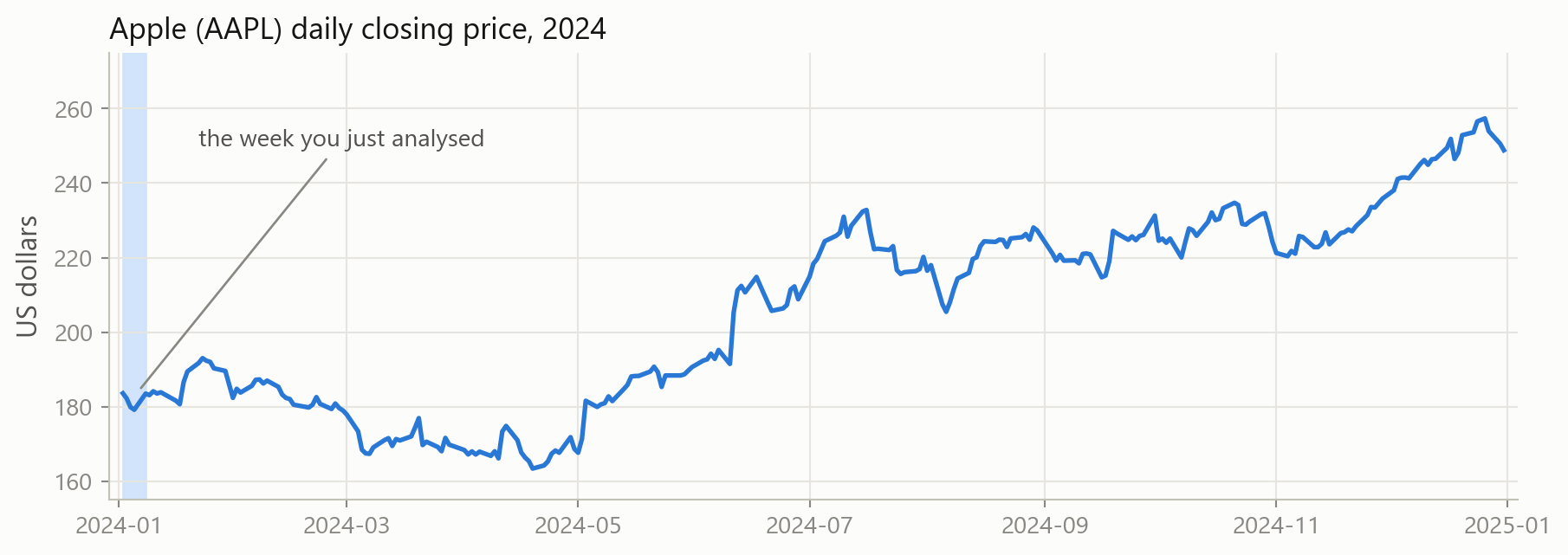
252 trading days; our five are the shaded sliver. Doing a whole year by hand would be painful, which is why Session 3 brings in pandas.
The Analyst’s Notebook: one investigation, a part after most sessions, done at home.
You are a junior analyst building a risk report on a small universe of US stocks. The running question:
How much do these stocks move, how does that differ across them, and could that movement be predicted at all?
By Session 4 you will have framed that question precisely, with real data. From Session 5 on, you build the models that answer it.
| data | your tools | |
|---|---|---|
| Part 1 · today | Apple & Coca-Cola, 2024 daily closes | lists, indexing, returns |
| Part 2 | the same, measured properly | functions, loops, dictionaries |
| Part 3 | 11 stocks, 2015–2024 | pandas tables and plots |
| Part 4 | the same, as a prediction problem | features, targets, evaluation |
| Parts 5 and 6 | next month’s volatility, forecast | cross-validation, ridge and lasso |
| Parts 8 and 9 | a warning before a big move | classification, thresholds |
| Parts 11 and 12 | the forecast and the warning again | trees, forests, boosting |
No live downloads: every price ships with the course. Results are identical for everyone. Sessions 7, 10 and 13 are case lectures of their own, with no part.
session_01_case.ipynb, 10 questions, done at home before Session 2:
Hints and full solutions are folded into the notebook. Work first, then check.
Runtime state Cells share a memory; “correct” means correct top-to-bottom from a fresh start.
Variables = assigns a name to a value; assigning again overwrites.
Types int, float, str, bool; and "150" is not 150.
Formatting f"{r:.2%}" and f"{p:.2f}": the two recipes we reuse.
Functions & methods round(x, 2) versus ticker.upper(): the dot-grammar runs the course.
Lists Index from 0, [-1] is the end, slice [a:b] excludes b.
Errors Read the last line first. Nothing is broken.
Simple return (p1 - p0) / p0: the object this course is about.
Without running anything, what does each line produce? (a value, or which error?)
Answers on the next slide; argue with your neighbour first.
| expression | result | |
|---|---|---|
| 1 | a[3] |
IndexError: positions are 0, 1, 2 |
| 2 | "5" + "5" |
"55": strings glue |
| 3 | a[-1] > 25 |
True: 30 > 25 |
| 4 | share_count |
NameError: never assigned |
| 5 | a[1:3] |
[20, 30]: stop excluded |
jobo@econ.au.dk. Stuck over 15 minutes? Note it and bring it next session.
Next session: functions, loops, and dictionaries, the tools that let you repeat a calculation over hundreds of prices at once instead of by hand.
Now, together
Opening Google Colab, saving your own copy, and running your first cells, live.