Machine Learning in Finance · Session 2
Last session you stored prices in a list, indexed it, and computed a simple return from two prices. That return is a single line:
That is the return for one day, from the first close to the second.
To study a stock you want every day’s return. Apple traded about 252 days in 2024, so that is 251 returns.
Writing them out one line at a time, (prices[1] - prices[0]) / prices[0], then (prices[2] - prices[1]) / prices[1], and so on, is not realistic.
You need a way to say: do this once for every day. That is a loop, and it is where we start today.
By the end of this session you can:
And you continue the course case: turning last session’s rough risk gauge into a real one.
Part 1
Doing something once for every item in a list.
Step through it one click at a time. Watch the highlighted line, and how the variable and the output change:
Now run it for real. Instead of printing prices one by one, let Python walk the list:
for price in prices: reads as “for each price in the list”. The indented line runs once per item.
Each time round, price holds the next value in the list:
price is an ordinary variable, and you choose its name.
Python knows what is inside the loop from the indentation:
The colon : opens the loop; the indented lines below it are its body.
Before running, decide how many lines this prints, and what they are.
One line for each item, or something else? Press Run to check.
A loop can build a running total. Start at zero, then add each price:
This is exactly what sum(prices) does. Now you can see inside it.
That shape comes up constantly:
0 for a sum)Set up, then loop and update, then use the result. Summing, counting, and averaging all follow this one pattern.
+=Updating a variable from itself, total = total + r, is so common that Python gives it a shorthand:
total += r means total = total + r. The same works for -=, *=, and /=. We will use it for accumulators from here on.
range(n) gives the whole numbers 0, 1, ... , n - 1 to loop over:
Use it when you care about positions, not the values themselves.
range(start, stop) begins at start and stops before stop:
Just like slicing, the stop value is not included.
To compare each day with the one before it, loop over positions and use i and i - 1:
Starting at 1 means the first pair is day 2 against day 1. There is no day before day 1.
To collect results, begin with an empty list and grow it with .append:
[] is a list with nothing in it yet. This is how you gather values as a loop runs.
Put the two ideas together: loop over positions, and append each return:
Five prices give four daily returns. The same formula as last session, now applied to the whole list.
Use a loop to add up all the returns into total. Start total at zero, and add each return inside the loop.
The accumulator pattern, on the returns:
Result: 0.011. Start at zero, add each return once, read the total after the loop.
Part 2
Running code only when a condition is true.
Last session a comparison gave True or False. if acts on that answer:
The indented block runs only when the condition is True. Change price to 240 and run it again.
else handles what happens when the condition is False:
elif (short for else-if) adds further cases, checked in order:
What does this print? Decide before you run it.
Which branch is true when r is exactly zero?
Put the two together: check a condition for every item. Count the up-days:
The if sits inside the loop body, indented once more. up_days grows only on positive days.
Each : opens a block, indented one step further than the last:
Read the indentation to see what belongs to what.
Count how many returns were negative (a down day).
The up-day count, with the comparison flipped:
Result: 2. Two of the five returns are below zero.
Part 3
Repeating for as long as a condition stays true.
A for loop runs once per item. A while loop runs for as long as a condition holds, however many times that takes.
How many years to grow 100 into 150 at 10% a year?
You did not have to know the answer in advance. The loop keeps going until value reaches 150.
Step through it. The condition is checked before each pass; watch value and years change:
Something inside the loop has to move the condition towards False, or it runs forever:
A while loop needs an exit. Make sure each pass changes something the condition depends on. If a cell seems stuck, interrupt it with the stop button.
How many years to grow 1000 into 1500 at 8% a year? Complete the while loop.
Two lines in the body: grow value, then count the year.
Result: 6. After five years the value is still under 1500; the sixth year pushes it above.
Part 4
Naming a calculation once, so you can reuse it anywhere.
print, len, max, and sum are functions: a name, then inputs in brackets. Today you write your own.
def creates a function. You give it a name, its inputs, and what it returns:
def name(parameters): opens the functionreturn hands a value back to whoever called itOnce defined, a function can be used again and again:
Write the formula once, and trust it everywhere. There is no copy to get wrong.
The names in the def are parameters; the values you pass in are arguments:
Inside that call, p0 is 100 and p1 is 110.
Without return, a function does its work but gives nothing back:
x is None: show printed a value but did not return one. Use return when you want to keep the result.
simple_return needs two inputs. What happens if you give it only one? Predict, then run.
Python will not guess the missing value.
A parameter can have a default, used when you do not pass it:
rate=0.05 in the def sets the default. Passing a value overrides it.
A docstring is a short description in triple quotes, just under the def:
Your editor shows the docstring when you hover over the function, and help(...) prints it. A one-line note now saves confusion later.
Functions and loops combine. Here is the average of a list, as a function:
The name average now stands for four lines of work.
Write a function total_return(prices) that returns the return from the first price to the last.
The first price is prices[0], the last is prices[-1].
Result: 0.10. The function works for a list of any length, because prices[-1] is always the last one.
Part 5
Storing values by name, instead of by position.
A list finds a value by its position, prices[0]. A dictionary finds a value by a key you choose, such as a stock’s name.
Curly braces, holding key: value pairs:
Here the keys are tickers, and the values are their yearly returns.
Use the key in square brackets, the way a position works for a list:
A key like "AAPL" is usually clearer than a bare number such as [0].
Assign to a new key to add a pair; assign to an existing key to change it:
A for loop over a dictionary walks its keys:
ticker takes each key in turn, and year_return[ticker] reads its value.
Values can be anything, including whole price series:
One object now holds every stock’s prices, each under its own name.
Add Coca-Cola’s volatility of 0.011 to the dictionary, then read it back.
Result: 0.011. Assigning to a new key adds it; looking it up reads it back.
Part 6
Everything from today, combined into a real measure of risk.
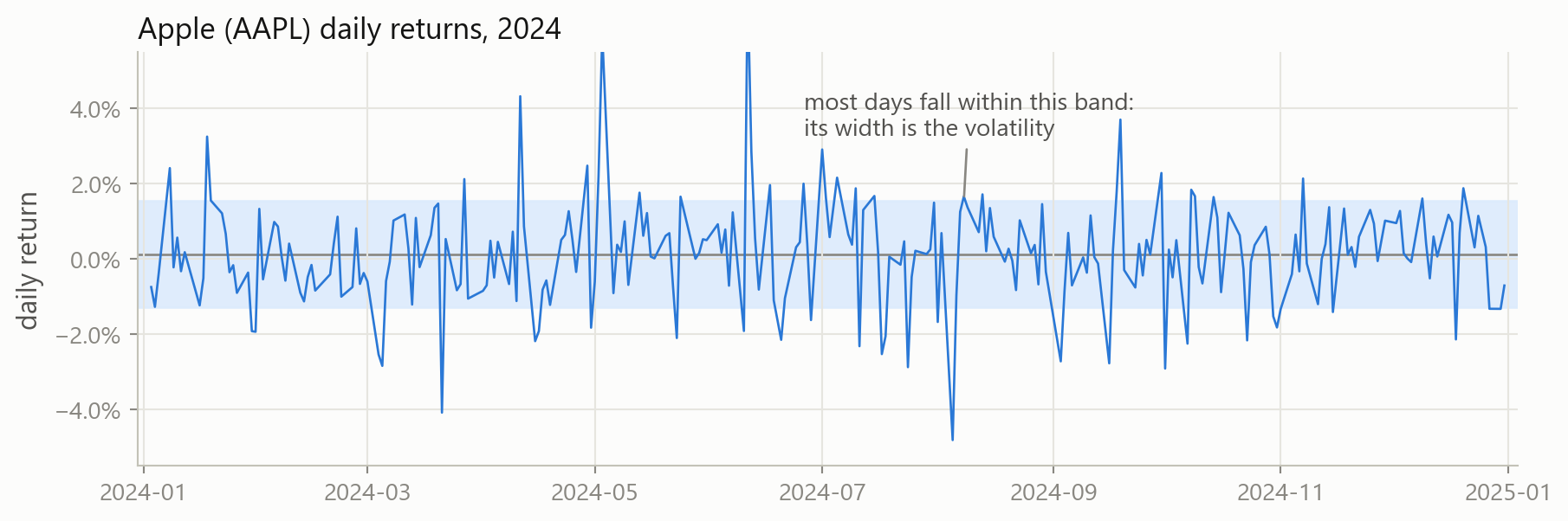
Last session’s risk gauge used only two days, the highest and the lowest. A better measure uses every day’s return. That measure is volatility: how much the daily returns typically spread around their average.
Volatility is the standard deviation of the daily returns:
\[ \sigma = \sqrt{\ \frac{1}{n}\sum_{i} \left(r_i - \bar{r}\right)^2\ } \]
In words: take each return’s distance from the average, square it, average those squares, and take the square root. It is the typical size of a daily move.
Each step is something you can already do:
sum(returns) / len(returns)** 0.5We now build these into one function, one step at a time.
Start the function with just step 1, the returns loop. It is not finished yet:
So far it only collects the daily returns into a list.
Add step 2, the average return. Still not finished:
Now it also has the average of those returns.
Add step 3, the spread, and return it. Now it is complete, so run it:
Every idea from today is here: two loops, an empty list, +=, and a return.
Now reuse the function. Give it Apple’s week of prices:
This calls the volatility function defined on the previous slide.
The same function, a different list:
Coca-Cola’s real closes for the same five days. A much smaller number than Apple’s: this price moved less from day to day.
Keep both answers together, each under its ticker:
Apple’s number is the larger one. This is the volatility comparison the case asks you to build.
Each point is one day’s return. Volatility is the width of the band they mostly fall inside.
For loops for x in items: runs the body once per item.
While loops while condition: repeats until the condition is false.
if / elif / else Run a block only when a condition holds.
Functions def name(args): with return, plus defaults and a docstring.
Dictionaries {key: value}, looked up by key, not position.
Volatility The standard deviation of the daily returns.
The risk report continues. Last session you compared Apple and Coca-Cola with a rough price range. This session you replace it with a proper measure:
Build a volatility calculation from the daily returns, run it on each stock, and organise the results in a dictionary. Still no pandas: just today’s loops and functions.
session_02_case.ipynb, done at home before Session 3:
Hints and full solutions are folded into the notebook. Work first, then check.
session_02_exercises.ipynb: loops, if, while, functions, and dictionaries. Hints and solutions folded in.
jobo@econ.au.dk. Stuck over 15 minutes? Note it and bring it next session.
Next session: packages. pandas, numpy, and matplotlib do all of this on eleven stocks at once, and plot the results.