Annualised volatility, in percent. Three lines of pandas.
A question that ranking cannot answer
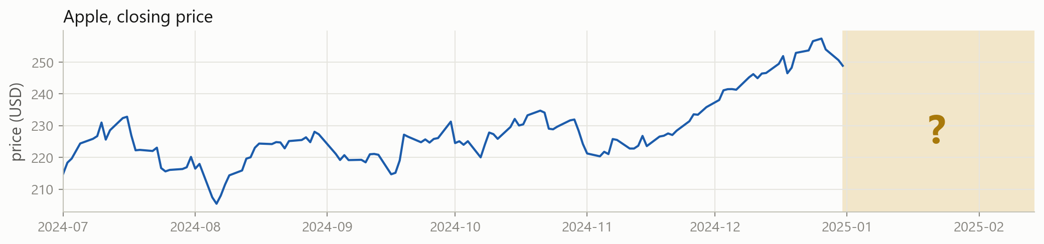
Will tomorrow be an up day? Nothing you have written so far even attempts this. Every tool from Sessions 1 to 3 describes data that already happened.
Describing, and predicting
Describing
What did happen?
Apple’s volatility was 28.4% a year
Nvidia moved most, Coca-Cola least
The worst day was 16 March 2020
You can check every one of these against the data.
Predicting
What will happen?
Tomorrow’s return will be about +0.3%
This client will default
This filing is unusual
You cannot check any of them yet. That is the whole problem.
Today
A prediction needs four things: a table of the right shape, a rule, a way to score the rule, and data the rule has never seen. Today is those four things.
By the end of the session you can:
put a problem into the statistical learning framework
tell supervised from unsupervised, regression from classification
handle missing values, extreme values and columns on different scales
score a prediction with MAE, MSE, RMSE, R² or a confusion matrix
explain overfitting and the bias-variance trade-off to somebody else
This session is part maths
Sessions 1 to 3 were about writing code. This one is mostly about ideas, and ideas here are written in symbols.
Nothing today is new maths. It is the vectors, matrices and sums you already use in econometrics, written the way machine learning writes them, plus the occasional expectation.
We still write code, and there are live cells throughout. But we do not fit a model today. That starts in the next block, once the ideas are in place.
1 · The statistical learning framework
Part 1
Observations, features, targets, and the error nobody can remove.
It all starts with one table
Each row is one observation. Each feature column is something you know at that moment. The target column is what you want to predict.
The same objects, three vocabularies
You already know most of these words. Machine learning just uses different ones.
econometrics
machine learning
in this table
observation
sample, instance, example
one row, one date
independent variable, regressor
feature, predictor, input
ret_1d, vol_20d
dependent variable
target, label, response, output
ret_next
coefficient
weight, parameter
one number per feature
residual
error
what the rule got wrong
model
learner, estimator
the rule itself
Building that table, from prices
shift(-1) pulls tomorrow’s return back onto today’s row. Every feature on a row is known before the target happens. That is the rule that makes the table honest.
n and p
The table has a standard notation, and it is the notation from Session 3.
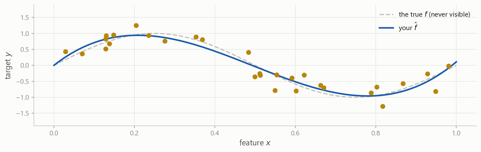
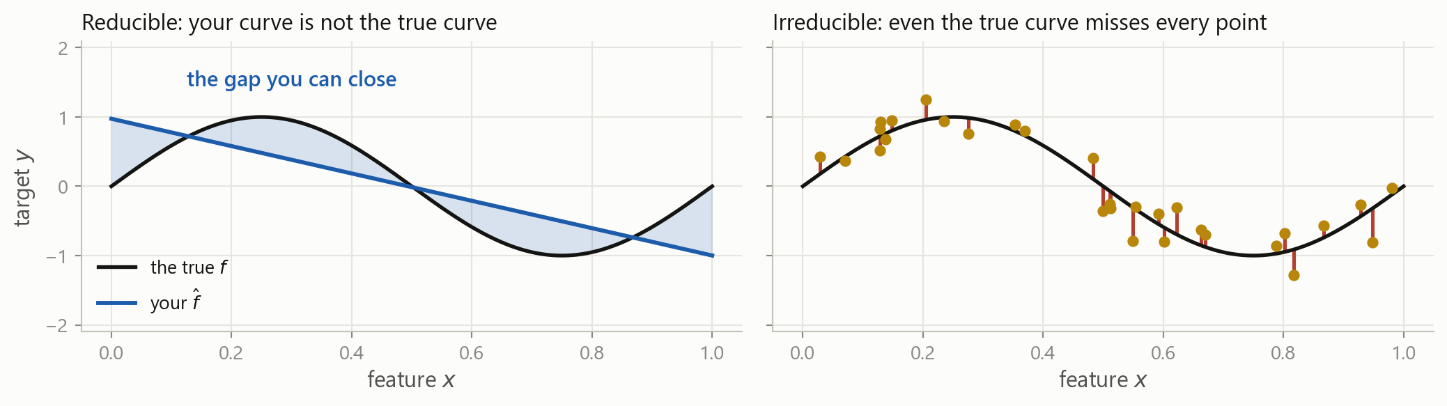
The gap between your estimate and the truth. Better features, more data or a better model shrink it.
Irreducible
The noise itself. No model, no data and no amount of compute removes it. It is a property of the problem.
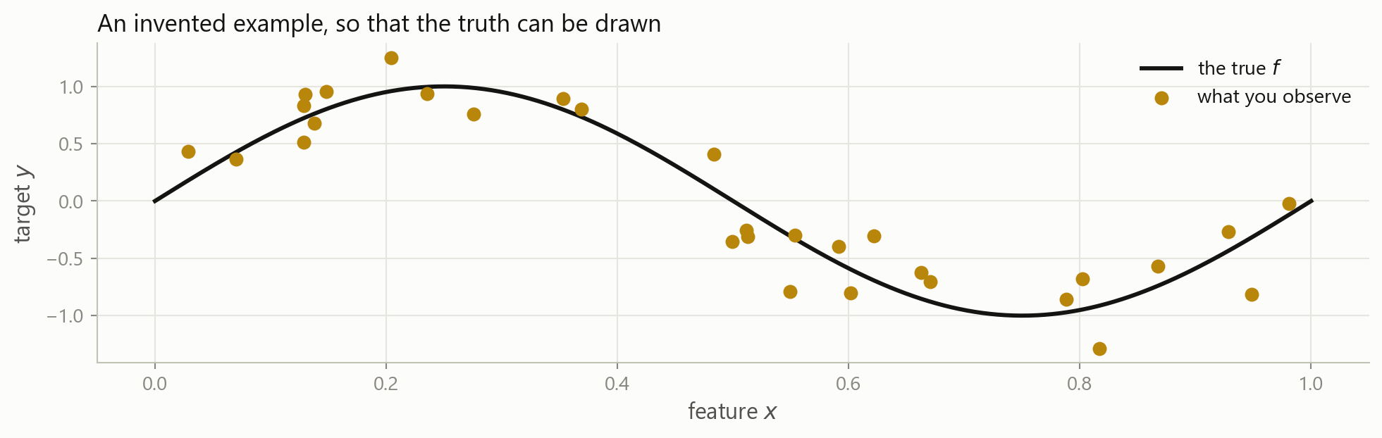
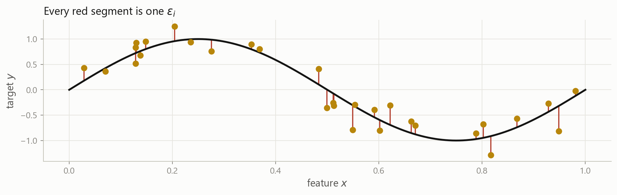
The floor, drawn
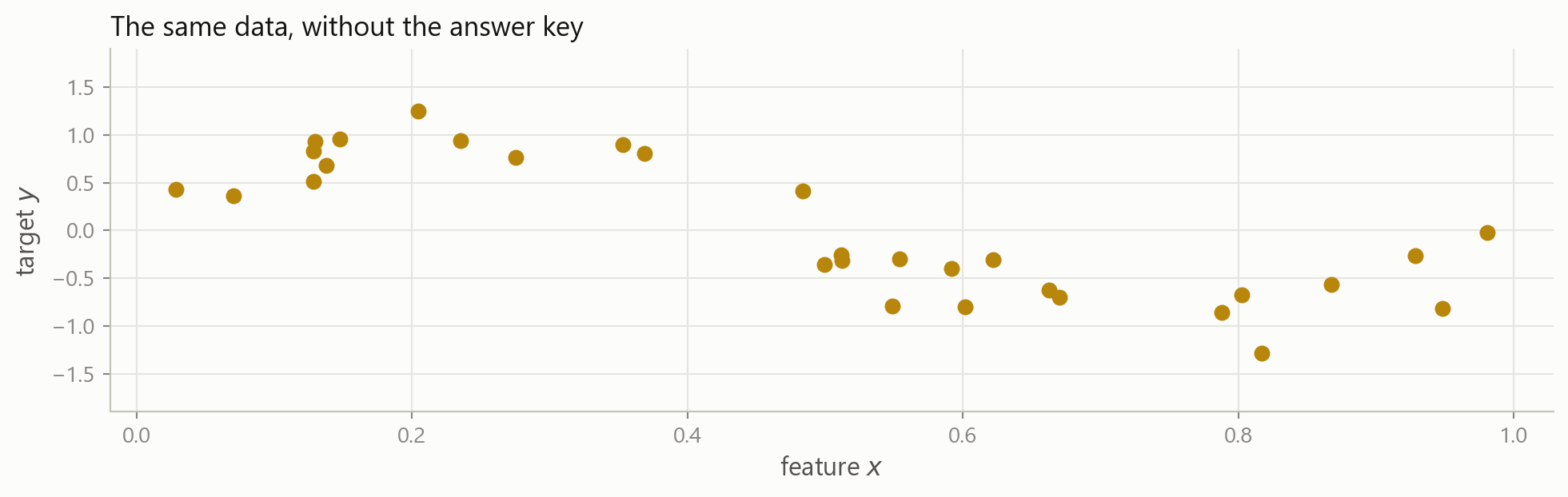
You can move the blue curve until it lies on top of the black one. The red segments would still be there, because they are the \varepsilon from earlier: the part of y that no feature in your table accounts for.
In finance the floor is high
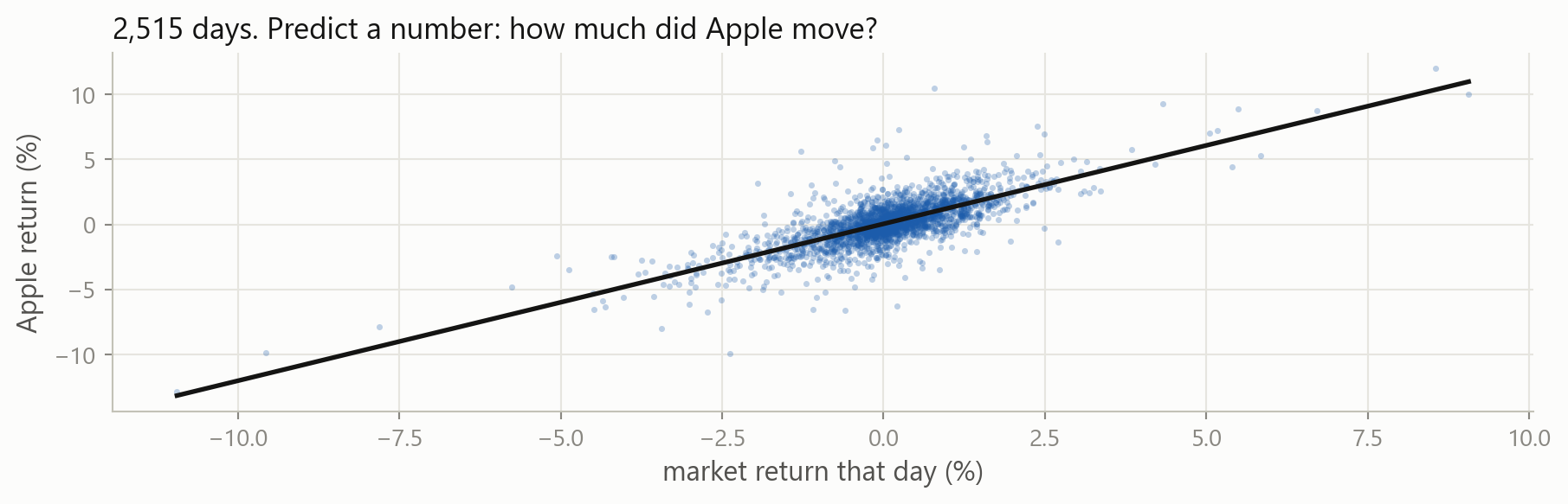
0.56
R² of Apple’s return on the market’s, same day
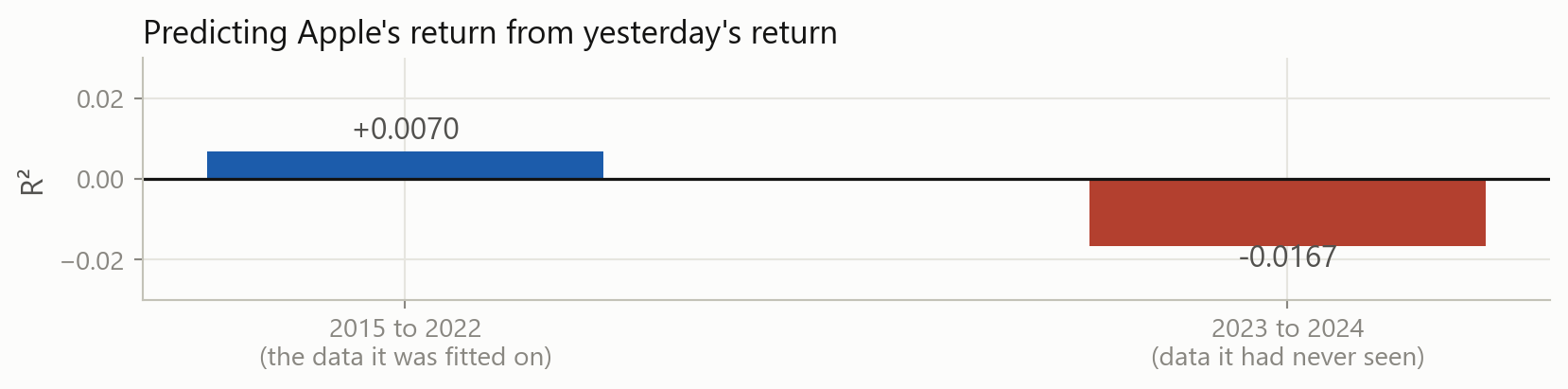
0.01
R² of Apple’s return on yesterday’s return, in sample
-0.02
the same rule, on data it had not seen
Explaining today with today is easy. Explaining tomorrow with today is close to impossible, because \operatorname{Var}(\varepsilon) is enormous.
That last number is not a typo. We come back to it in Part 4.
Linear regression is a machine learning model: a rule with parameters, chosen to fit a sample. It is the simplest one, and it is still the one to beat.
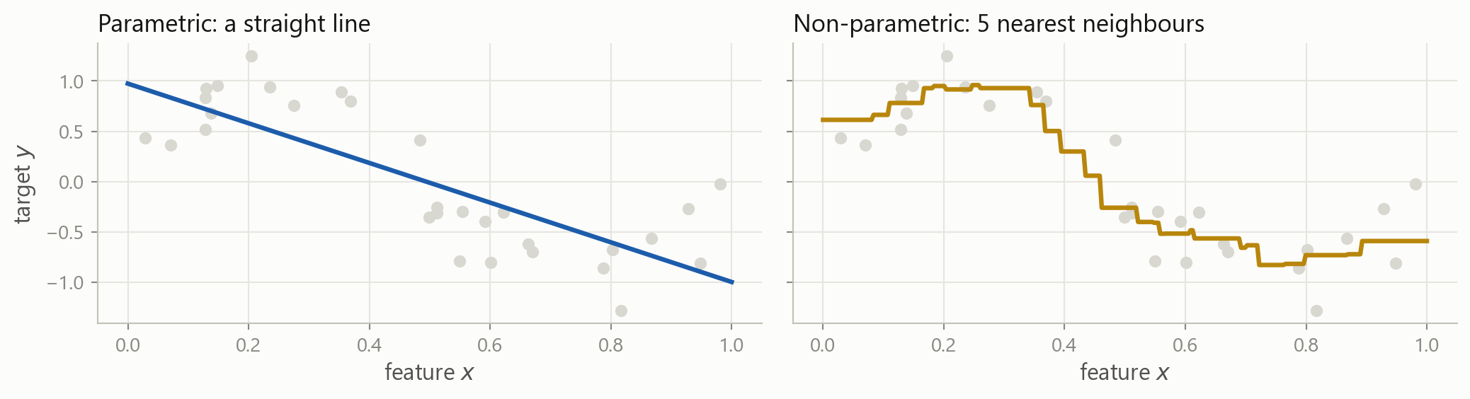
Assume a shape, or do not
Parametric
Pick a form first, then find its numbers.
Linear regression fixes one coefficient per feature, plus an intercept, whatever the sample size.
Cheap, stable, easy to read. Wrong if the true shape is not that shape.
Non-parametric
Let the data choose the shape.
Nearest neighbours, trees, splines. The rule grows with the sample.
Flexible. Needs far more data, and is harder to explain.
The same data, both ways
Two shapes for the two coefficients you get on the left. On the right there are no coefficients at all: the rule is “average the five closest rows”.
The rows you learn from, and the rows you check on
A model has already seen the answers in the rows it was built from, and a flexible enough rule can simply memorise them. So a score computed on those rows is not evidence of anything.
Why you split is today’s business, and it runs through the rest of the session. How to split well, and how to reuse the training rows without ever touching the test rows, is model selection and cross-validation in the next block.
Your turn 1
rets["MSFT"] is a Series of daily returns. Build a two-column table whose target is the return five days ahead.
A negative shift moves the future backwards onto today’s row. Shifting the wrong way gives you yesterday’s return as a target, which you could predict perfectly and which would be worth nothing.
2 · What kind of problem is it?
Part 2
Supervised, unsupervised, and the one we are not covering.
One question decides almost everything
Supervised: you have the answers
For every row in the training data, somebody has already written down the target.
Creditpast loans, and whether each one defaulted
Tradingpast days, and what the return turned out to be
Fraudpast transactions, and which were later confirmed as fraud
Ratingspast issuers, and the rating each was given
The target column is the expensive part. Somebody had to observe it, or label it by hand, and there is usually far less of it than you would like.
Regression: the target is a number
The answer can be any value on the vertical axis. This is the OLS picture you already know, seen as a prediction problem.
Classification: the target is a label
Now there are only two possible answers, and being “nearly right” is not a thing.
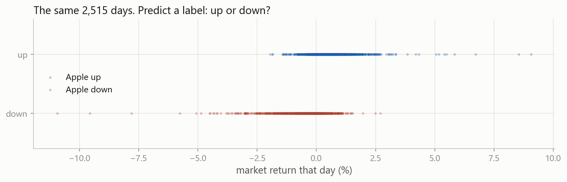
The same data, two different problems
Nothing changed in the data. You chose what the target would be, and that choice changes the model you can use, the metric you score it with, and what a mistake costs you.
As regressionpredict the return, then act on its size
As classificationpredict the direction, then act on the direction
Turning a number into a label always throws information away. A +0.02% day and a +6% day become the same “up”. Sometimes that is the right trade, because direction is easier to get right than size.
Making the label yourself
A comparison gives True and False, and .astype(int) turns them into 1 and 0. 53% of days are up, which will matter a great deal when we start scoring classifiers.
Unsupervised: nobody wrote the answers down
There is no target column. You have \mathbf{X} and nothing else, and the question becomes “what is the structure in here?”
Clusteringwhich of these stocks behave alike, without being told the sectors
Dimension reduction500 correlated series, and three factors that carry most of it
Anomaly detectionwhich trades do not look like any of the others
Topic modelswhat are these ten thousand filings about
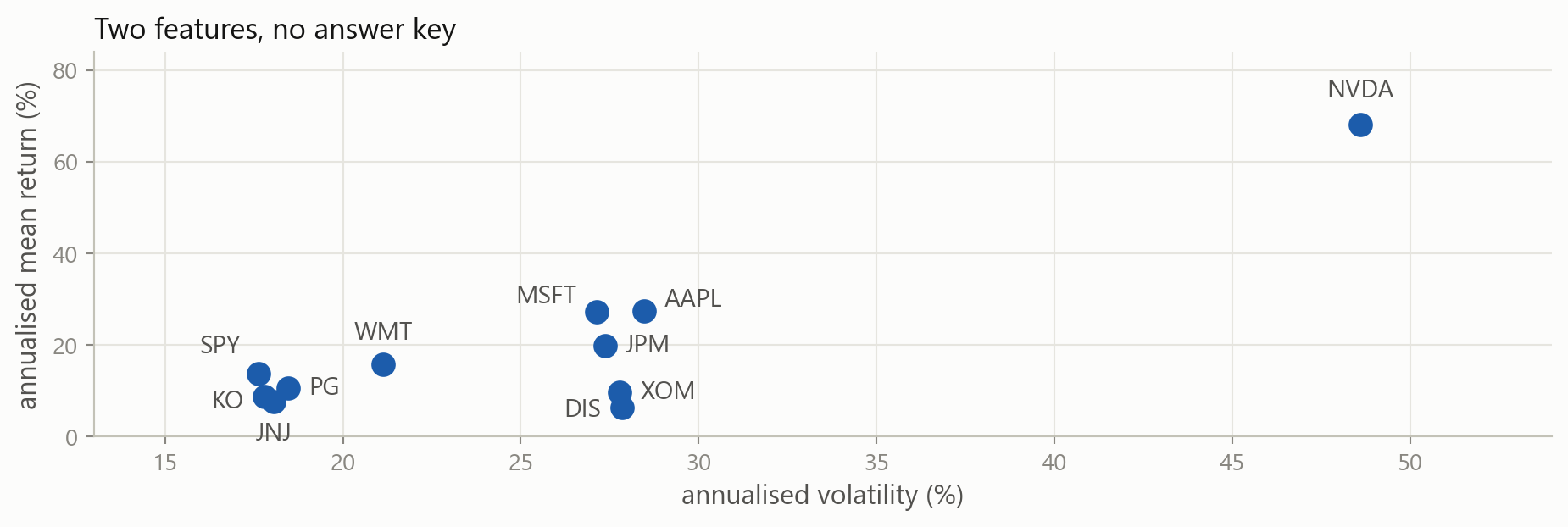
Eleven stocks, no target
Nobody labelled these. You can still see that the defensive names sit together in the bottom left, and Nvidia sits alone. That is clustering, done by eye.
The catch with unsupervised work
Supervised
There is a right answer, so there is a score.
You can say “this model is better than that one” and defend it with a number.
Unsupervised
There is no right answer, so there is no score.
Three clusters or five? Both are defensible. You are back to judgement.
This is why supervised learning dominates in practice, and why most of this course is about it.
Reinforcement learning
The third paradigm. No fixed table at all: an agent takes actions in an environment, gets rewards, and learns a policy that earns more of them.
In principleoptimal execution, hedging, market making, portfolio rebalancing
In practiceit needs an environment to practise in, and markets do not offer one
We do not cover reinforcement learning in this course. You should know the word, and know that it is a different setting: the data depends on what the agent decided to do.
Your turn 2
Which is each of these?
Predict a bond’s yield spread next month
Group 3,000 funds by how they behave, with no style labels
Decide whether a filing will be followed by a restatement
Compress 60 macro series into a handful of factors
Predict how many basis points a stock moves after an earnings surprise
Your turn 2: answer
Predict a spread ➜ regression, the target is a number
Group funds ➜ unsupervised, clustering, no target exists
Restatement or not ➜ classification, the target is a label
Compress 60 series ➜ unsupervised, dimension reduction
Basis points after a surprise ➜ regression, the target is a number
Number 3 could be made a regression by predicting the probability instead. The line is not always sharp, and the decision is yours to defend.
3 · Real data is never that shape
Part 3
Missing values, extreme values, and columns measured in different worlds.
Missing values, and where they come from
Calendars disagreeUS and European exchanges keep different holidays, so a merged table has gaps
The company was not therean IPO in 2019 has no 2015 rows, and a delisted firm has no 2024 rows
Trading stoppedhalts, suspensions, and days with no quote
Reporting is optionala fund reports until the month it would rather not
The last one is the dangerous one, and we come back to it.
Finding them
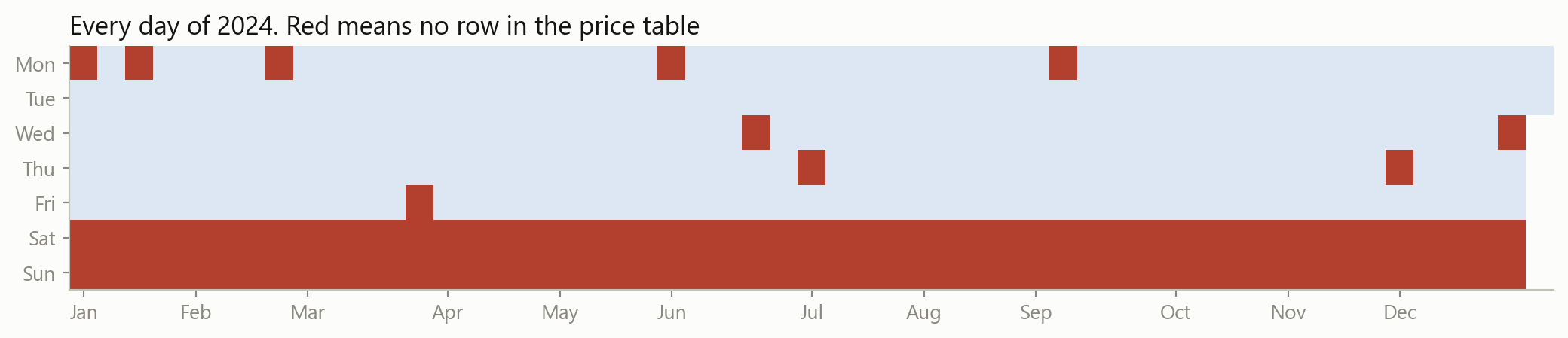
reindex forces the table onto a row per calendar day, which is what happens the moment you merge with anything daily. 1,136 of 3,652 days are now empty, and .isna().sum() counts them column by column.
A picture of it
Two solid rows of weekends, and ten single red squares: New Year, Martin Luther King Day, Presidents’ Day, Good Friday, and the rest of the market holidays. A picture of missingness usually tells you the cause immediately, which is what you need before you decide what to do about it.
Three ways out
Drop the rowsdf.dropna(). Safe when the gaps are few and unrelated to what you are studying.
Drop the columnif a feature is 60% empty it is usually not worth rescuing.
Fill them infillna, ffill, interpolate. You are inventing data, so be deliberate about it.
Keep the factadd a column that records “this was missing”. Sometimes that is the signal.
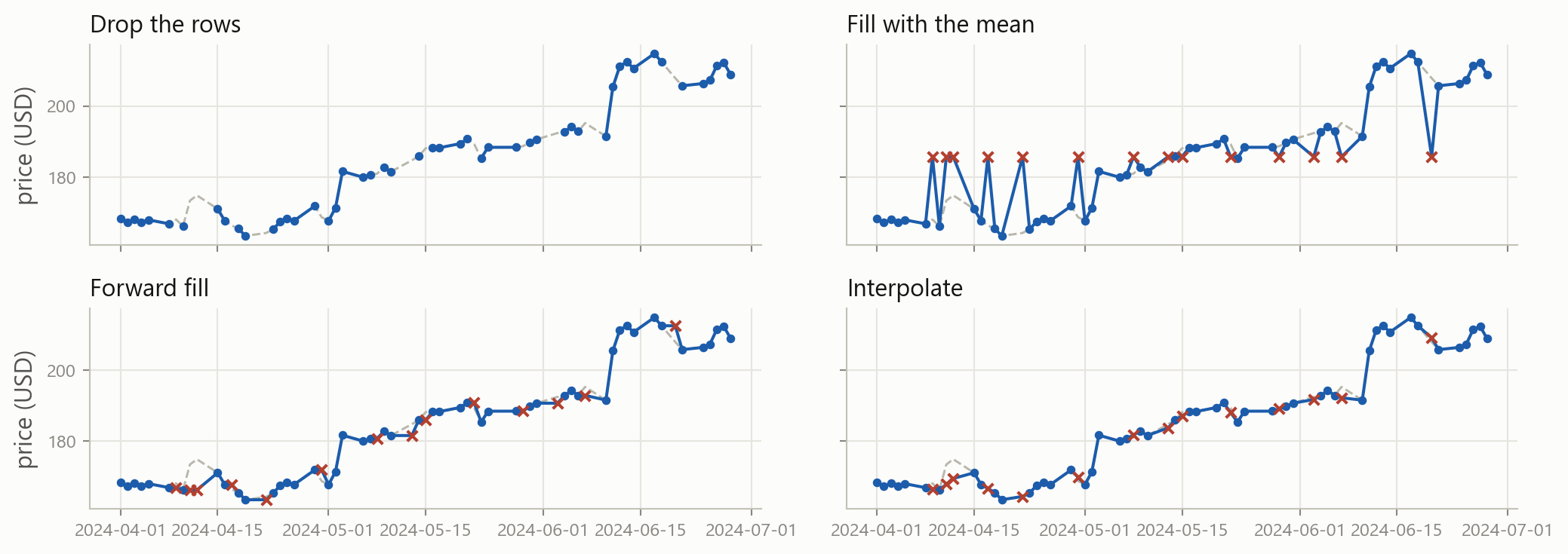
What each choice looks like
Grey dashed is the truth, red crosses are the invented values. Fourteen days removed from Apple’s spring.
The accurate answer is the illegal one
$10.86
mean error, fill with the column mean
$2.76
mean error, forward fill
$1.67
mean error, interpolate
Interpolation wins, because it draws a line between the price before the gap and the price after it.
Standing on 8 May you would not have known 9 May’s price, and that is the price the interpolated value is drawn from. Interpolation quietly puts tomorrow’s information into today’s row, and every result built on it is optimistic. Forward fill only ever looks backwards.
Why it is missing decides what you may do
Missing for an unrelated reason
Thanksgiving. A vendor outage. A field nobody filled in.
Dropping those rows costs you sample size and nothing else.
Missing because of the value
The fund stopped reporting after the month it lost 40%. The firm delisted because it failed.
Drop those rows and your sample is only the survivors.
The second case has a name in finance: survivorship bias. It is the reason a backtest on today’s index members looks so good.
Extreme values
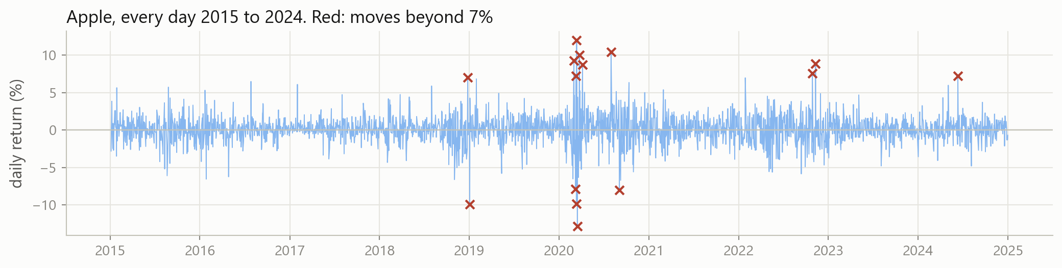
Most of them are in March 2020, and they are not mistakes. The best day was +12.0% and the worst was -12.9%, on the Friday and the Monday of the same weekend.
An error, or the whole point?
Probably an error
A price of 0, or of 1,000,000. A return of +4,000% because of an unadjusted stock split. A date in 1901.
Fix it or drop it, and write down what you did.
Probably the point
March 2020. The 2008 quarter. The day the takeover was announced.
Delete these and you have built a model of a market where nothing ever happens.
In most fields the extremes are noise. In finance they are usually the phenomenon. Risk lives in the tail, so removing the tail removes the subject.
Two rules of thumb, and their limits
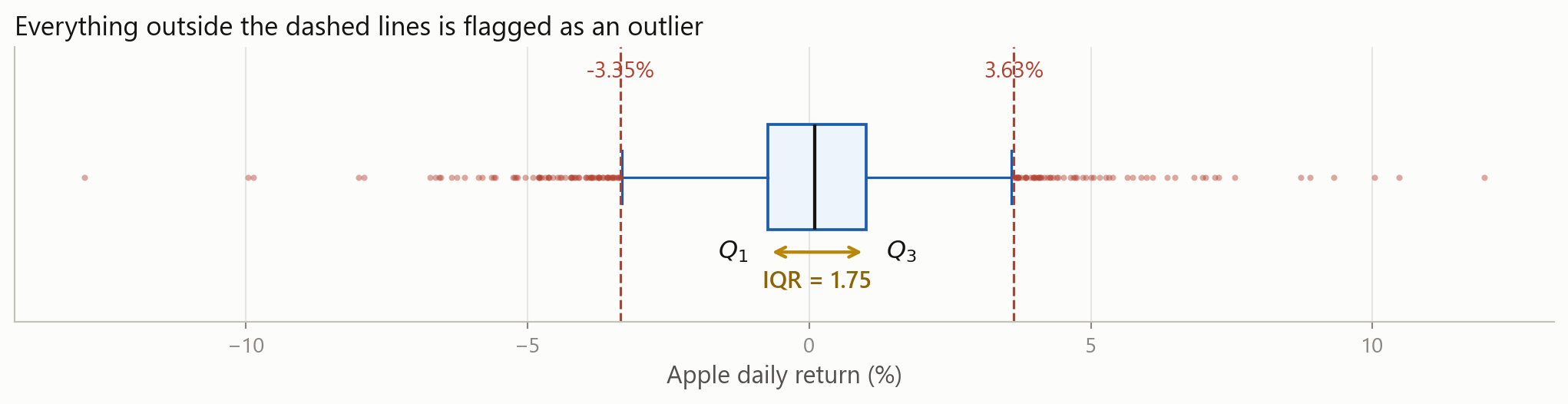
Q_1 and Q_3 are the 25th and 75th percentiles, and the interquartile range\text{IQR} = Q_3 - Q_1 is the width of the middle half of the data.
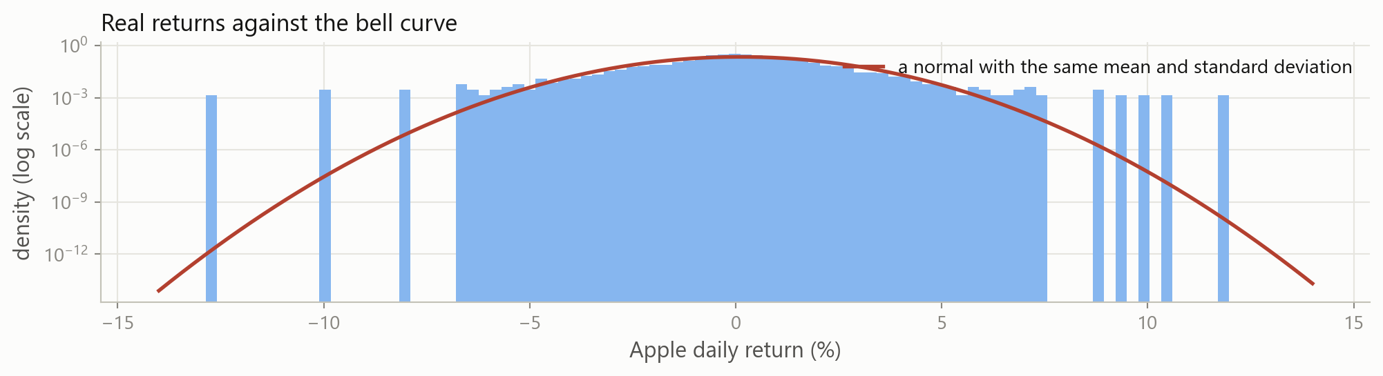
The rules assume a bell curve. Returns are not one, so the rules mark hundreds of perfectly real days as errors.
There is also a circular problem: one enormous day inflates s, which then makes that day look less extreme.
The tails are the whole story
The bars sit far above the red line at both ends. Days that “cannot happen” happen several times a decade, and they are the ones that decide whether a strategy survives.
So what do you actually do
Check the source firstmost true errors are visible in one plot or one .describe()
Do not delete by defaulta rule that flags 5% of your days is not finding errors, it is finding the market
Score with a robust metricMAE cares far less about one bad day than MSE does. Part 4.
Or transforma log squeezes the long right tail of prices, volumes and market caps
Whatever you choose, write it down. “We dropped returns beyond ±20%, three observations” is a sentence that belongs in the report.
Levels, and changes
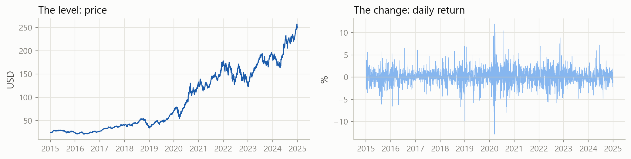
The left panel wanders off and never comes back, so its mean means nothing. The right panel hovers around a fixed level, so its mean and standard deviation describe something real. Model the changes, not the levels.
They add upa year’s log return is the sum of its days. Simple returns have to be compounded.
They are symmetric-50% then +100% gets you back to where you started, and in logs those cancel exactly
They tame right skewmarket cap, volume and price are all long-tailed, and a log makes them workable
They are nearly the samefor small daily moves, log(1 + r) and r agree to three decimals
Columns from different worlds
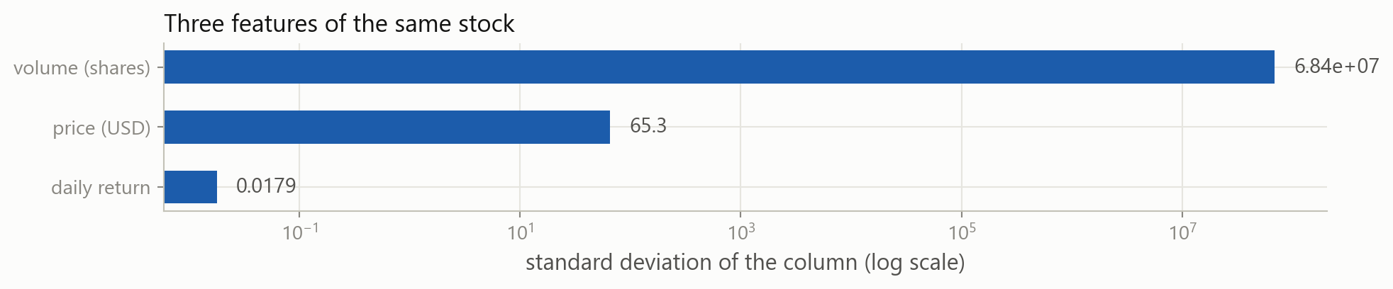
The volume column varies about four billion times more than the return column. Any method that measures distance, or penalises large coefficients, will hear only the volume.
Standardising
z_i = \frac{x_i - \bar{x}}{s}
Every column now has mean 0 and standard deviation 1, so a coefficient of 0.4 means the same thing in every column. OLS does not need this. Nearest neighbours, penalised regression and neural networks all do.
Columns that are not numbers
One column of text becomes one 0/1 column per category. This is one-hot encoding, and it is how a sector, a rating or a country gets into \mathbf{X}.
The rule that governs all of it
Every number you use to clean the data, the mean you filled with, the standard deviation you divided by, the quantiles you flagged outliers with, must be computed on the training rows alone.
Those are the rows from Part 1 that the model is allowed to learn from. Compute the mean over the whole sample instead and it already contains the period you were going to test on, so your test score flatters you and the model disappoints in production.
It is the same look-ahead problem as interpolating across a gap, and it is the single most common mistake in student projects and in published finance papers alike.
Your turn 3
Apply the IQR rule to Microsoft’s returns, and count how many days it flags.
134 days of 2,515, or 5.3%. Almost exactly what the rule flagged for Apple, and far too many to be errors. The fences sit at -3.2% and +3.5%, so the rule is calling an ordinary bad Tuesday an outlier.
4 · Was the prediction any good?
Part 4
Turning a column of mistakes into one number you can defend.
A rule, and what it predicted
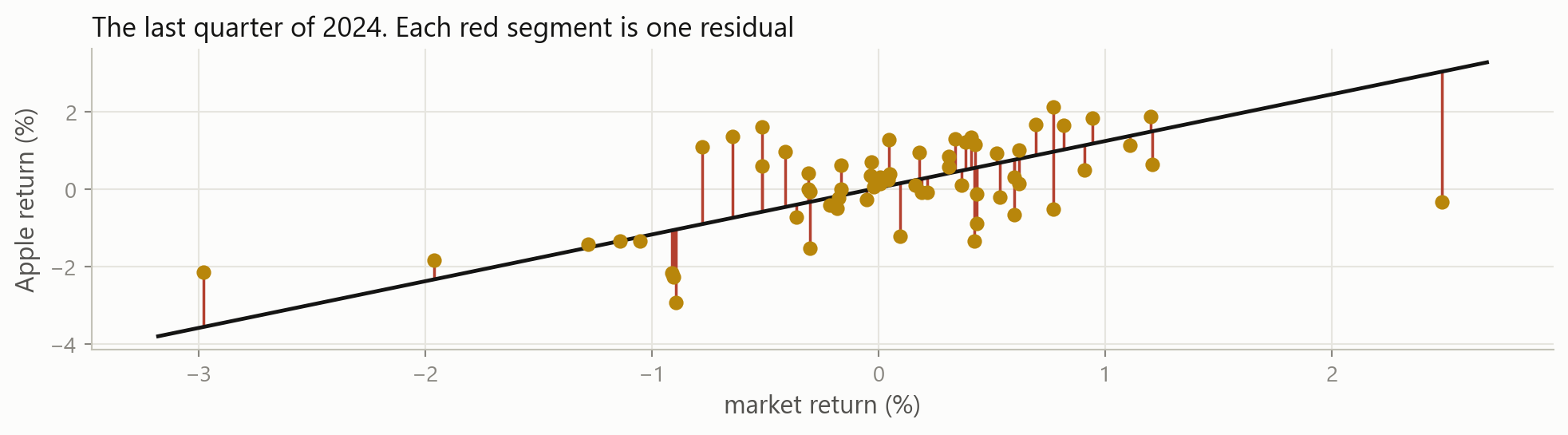
Session 3 fitted Apple’s return against the market’s and got two numbers. That is a model:
\hat{y}_t = 0.00043 + 1.2073 \, x_t
The residual
e_i = y_i - \hat{y}_i
Why you cannot just add them up
The average residual is four millionths. The average residual size is more than two thousand times bigger. Least squares picked the line that makes the positives and the negatives cancel, so the sum tells you nothing at all about how wrong the model was.
You need to remove the signs first. There are two standard ways to do that.
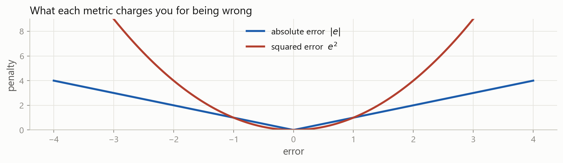
Squaring removes the sign too, but it also punishes a big miss much harder than several small ones.
MSE is in squared units, which nobody can interpret: 0.000142 squared returns. Taking the root puts it back into percent, which is why RMSE is the one you report.
All three, on the real residuals
RMSE is always at least as large as MAE. The gap between them tells you how uneven the errors are.
Why both exist
Being wrong by 4 costs four times as much as being wrong by 1 under MAE, and sixteen times as much under MSE.
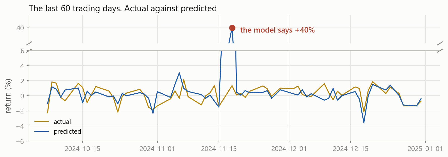
One terrible forecast
The damage, in numbers
×1.8
MAE, 0.75% to 1.38%
×5.1
RMSE, 0.99% to 5.09%
×26
MSE
One day in sixty. MAE says the model got a little worse. MSE says it fell apart.
Neither is lying. They answer different questions: “how wrong is this model on a normal day” and “how badly can this model hurt me”.
Percentage error is attractive because it has no units, and it is common in sales and demand forecasting.
Never use it on returns. A day where the true return is 0.0001 makes the denominator almost zero, so one ordinary day can contribute thousands of percent to the average.
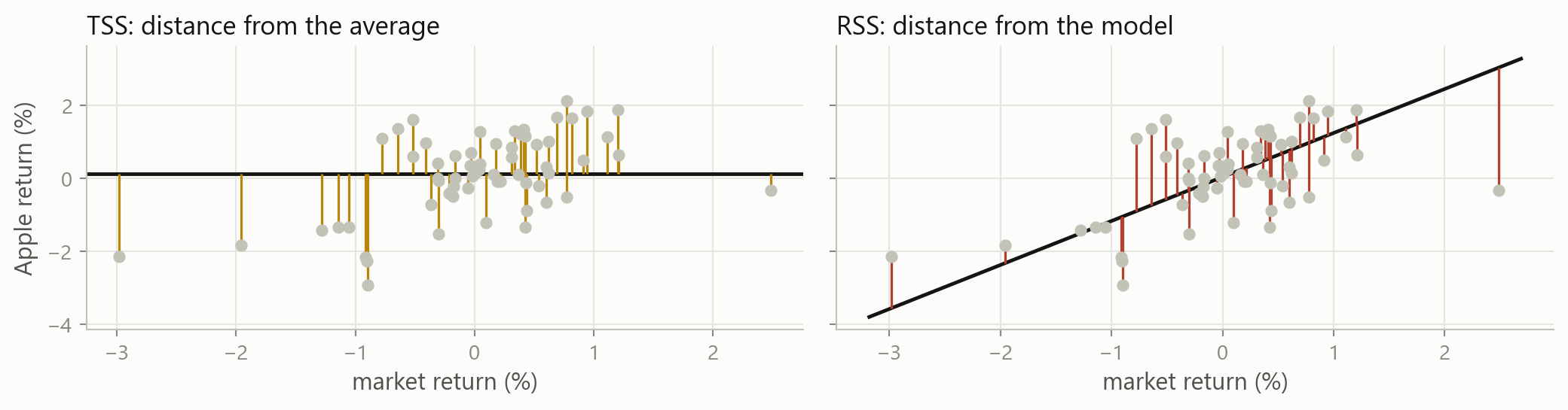
MAE and RMSE tell you how wrong you were. R² tells you how wrong you were compared with the laziest possible model: always predict the average.
R^2 = 0 means you matched that lazy model. R^2 = 1 means you fit every point exactly.
The two sums, drawn
R² is one minus the ratio of the red lengths to the amber ones, squared and added up.
R² on new data can be negative
Out of sample there is nothing forcing R² to be positive. Negative means you would have done better by always predicting the average.
And a tiny R² can still be worth a lot
An R² of 0.01 on next-day returns would be a serious result. It means 99% of what happens is noise to you, and the remaining 1%, applied every day across hundreds of names, is a business.
This is why finance is unlike most machine learning applications. A vision model with 1% explained variance is broken. A return model with 1% is a fund. Judge the number against the problem, never against 1.
Now change the target
Everything since the start of this part assumed the target was a number, so “how far off were you” had an answer. Change the target to a label and that question stops making sense: what is “up” minus “down”?
Regression, so far
predict Apple’s return from the market’s return
score it by the size of the residuals: MAE, RMSE, R²
Classification, from here
predict whether Apple rose, from whether the market rose
there is no residual, so score it by counting right and wrong
Same eleven stocks, same 2,515 days, same market feature. Only the target column changed, exactly as in Part 2.
Four things can happen
You said up, and it went upa true positive
You said up, and it went downa false positive, a false alarm
You said down, and it went upa false negative, a miss
You said down, and it went downa true negative
Every classification metric in use is built out of those four counts, and nothing else.
The confusion matrix
Predicting “Apple rose today” from “the market rose today”, over 2,515 days.
Counting them yourself
Four boolean masks and four sums. Nothing here that Session 3 did not already give you.
75.0% of days called correctly. It is the first number everybody computes, and on its own it is close to useless.
Where accuracy falls apart
Now predict something rare: a day when Apple falls more than 5%.
22
such days in ten years
99.1%
accuracy of a model that always says “no crash”
0
crashes it would ever warn you about
A model with no skill whatsoever beats almost anything you will build, measured by accuracy. When one class is rare, accuracy measures the class balance, not the model.
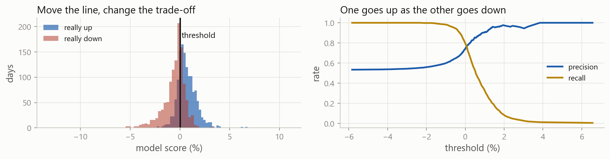
It catches 19 of the 22 crashes, a recall of 0.864. Before you celebrate, ask the other question: it warns on 278 days in total, so its precision is 0.068. Thirteen false alarms for every real one.
5 · Overfitting, and the trade-off
Part 5
Why the model that fits best is usually the one to throw away.
A model that is never wrong
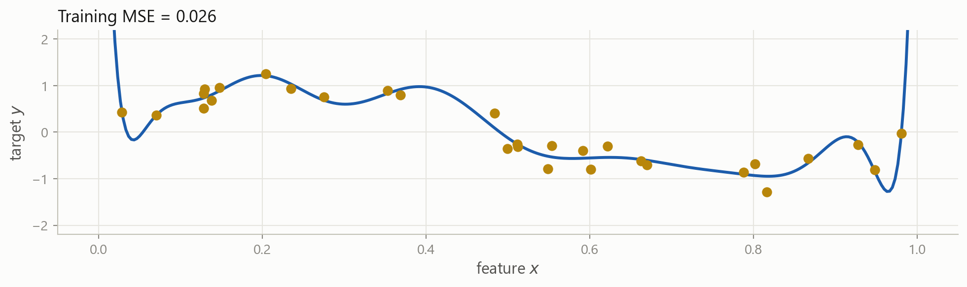
The same invented data from Part 1, and a curve that passes through almost every point. By every metric in Part 4, this is an excellent model.
So: is that the model you want?
Before the next slide, decide what you think.
What does this curve say will happen at x = 0.55?
If I collected thirty new observations, would it still fit them?
Which parts of that curve are the relationship, and which are the noise?
There is no trick. The answer is the whole of the rest of this session.
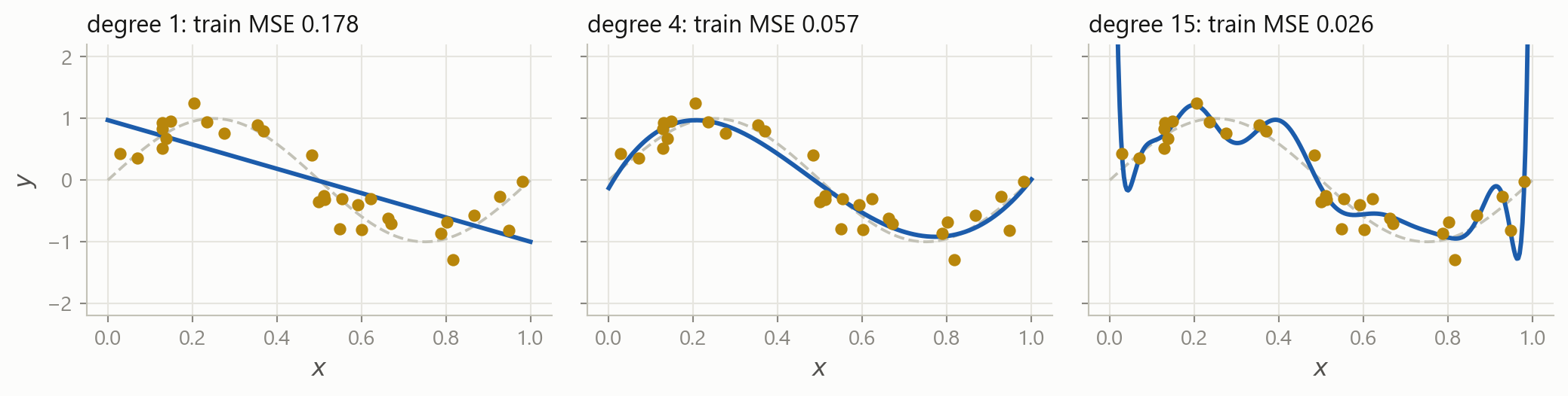
Three fits of the same thirty points
Grey dashed is the truth. Training error falls every time you add flexibility, and it will keep falling all the way to zero.
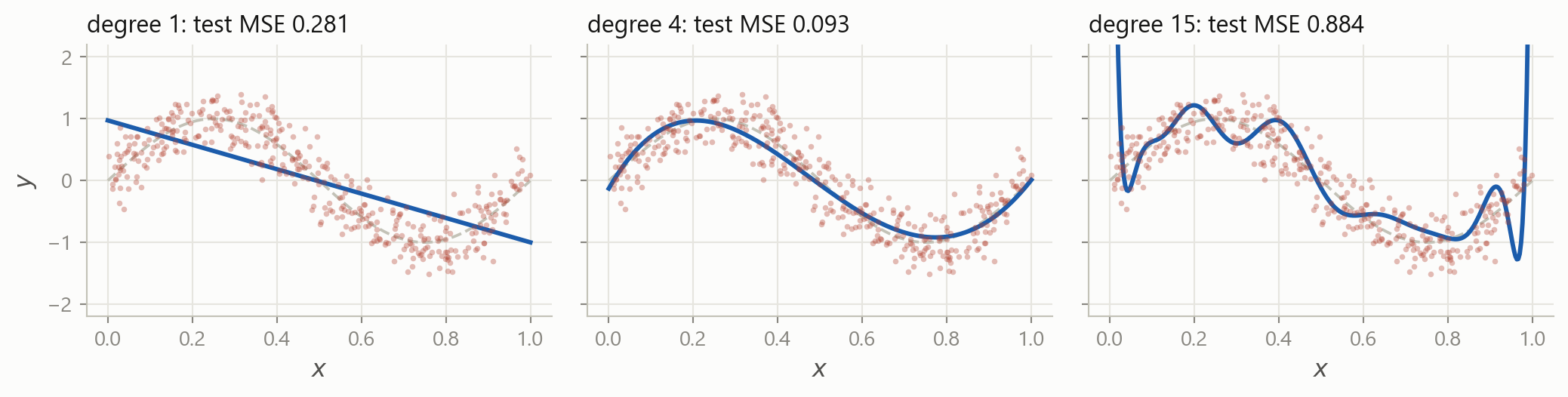
The same three, on data they never saw
Four hundred new points. The middle model is now the best by a distance, and the flexible one is thirty times worse than it was on its own training data.
Two ways to be wrong
Underfitting
The model is too rigid to represent the relationship.
Bad on the training data, bad on new data, and bad in the same way on both.
The straight line above.
Overfitting
The model has learned the noise as if it were signal.
Excellent on the training data, poor on new data. The gap is the symptom.
The degree-15 curve above.
You cannot tell them apart from the training score. That is the entire reason for everything on the next few slides.
The picture worth remembering
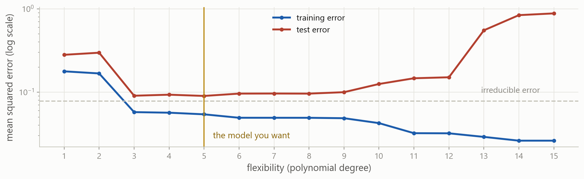
Training error falls forever. Test error falls, bottoms out, and then climbs. Every model selection procedure in this course is a way of finding that bottom without cheating.
Turn the dial yourself
x_train and y_train are the thirty invented points from a few slides back.
Which is why you held rows back
Training error kept improving all the way to degree 15. Test error stopped improving at 5. Only one of those two numbers was available while the curve was being chosen.
The rows you set aside in Part 1 are what turn “my model fits well” into evidence. Everything after today, cross-validation included, is a way of estimating that test error better without spending the test set.
Splitting the table
aapl is the feature table from Part 1. Splitting it is one line, because a DataFrame index knows about dates.
Time series break the usual rule
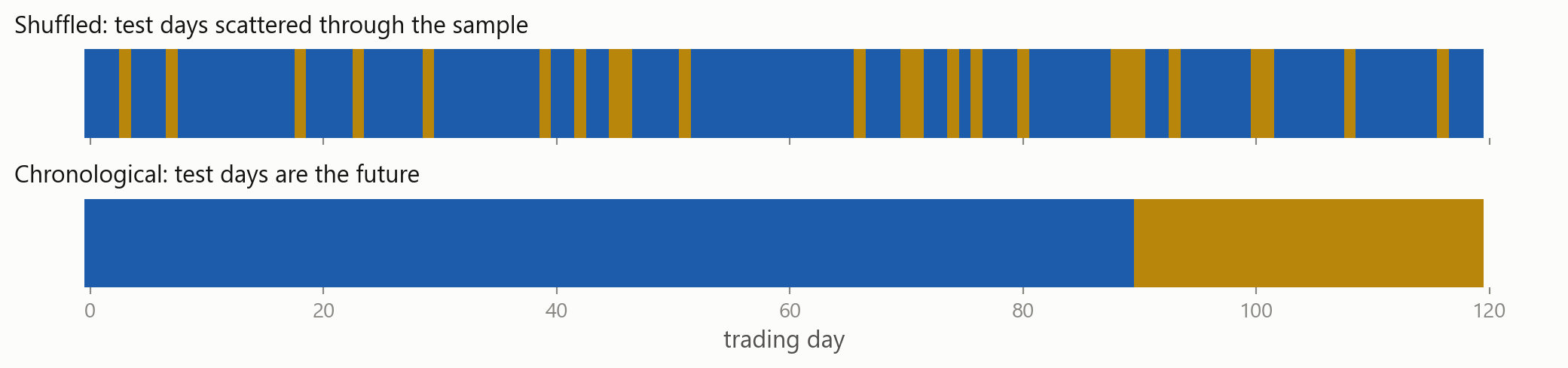
In the top panel the model trains on Wednesday and Friday to predict Thursday. It knows the future. Any backtest built that way will look wonderful and lose money.
The many faces of look-ahead bias
Shuffling a time seriesthe split has to be a date, not a random draw
Scaling on the full samplethe mean you subtracted contains the test period
Interpolating across a gapPart 3: the fill used the price after the gap
Choosing features after peekingyou tried forty ideas and kept the one the test set liked
Restated fundamentalsthe numbers in the database today are not the ones published then
Today’s index membersthe failures dropped out, so the sample is only the survivors
Where the error comes from
Test error is not one thing. Split it into two, and everything about model choice becomes clearer.
Bias
Error from the model being too simple to represent the truth.
It would still be there if you had a million rows.
Variance
Error from the model being too sensitive to the particular sample you drew.
Collect a different sample, get a different model.
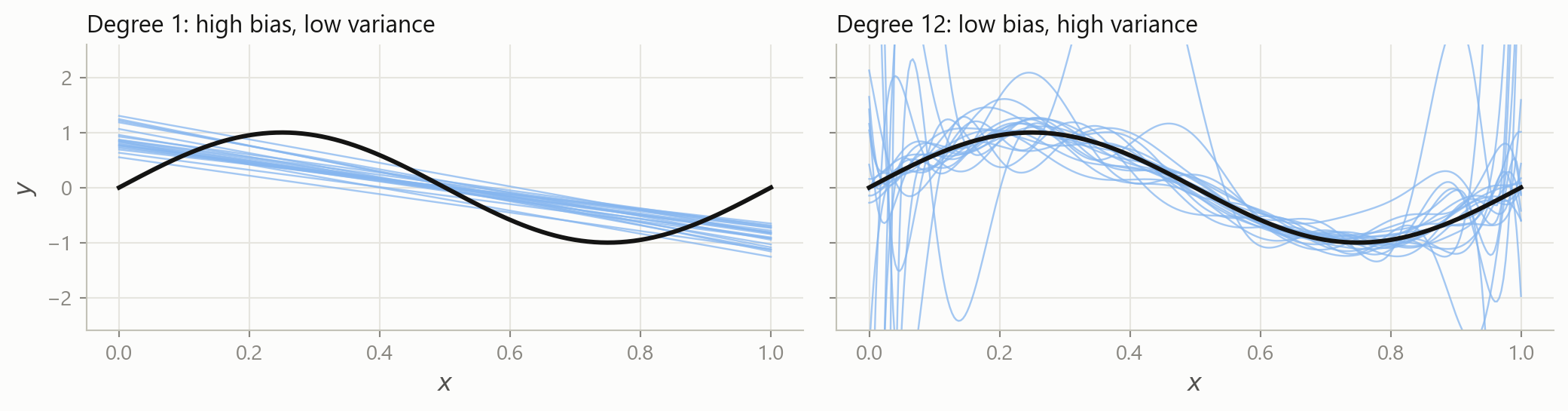
The same model, twenty different samples
Left: every line is wrong in the same way, and they all miss the curve. Right: the lines are right on average and wildly different from each other.
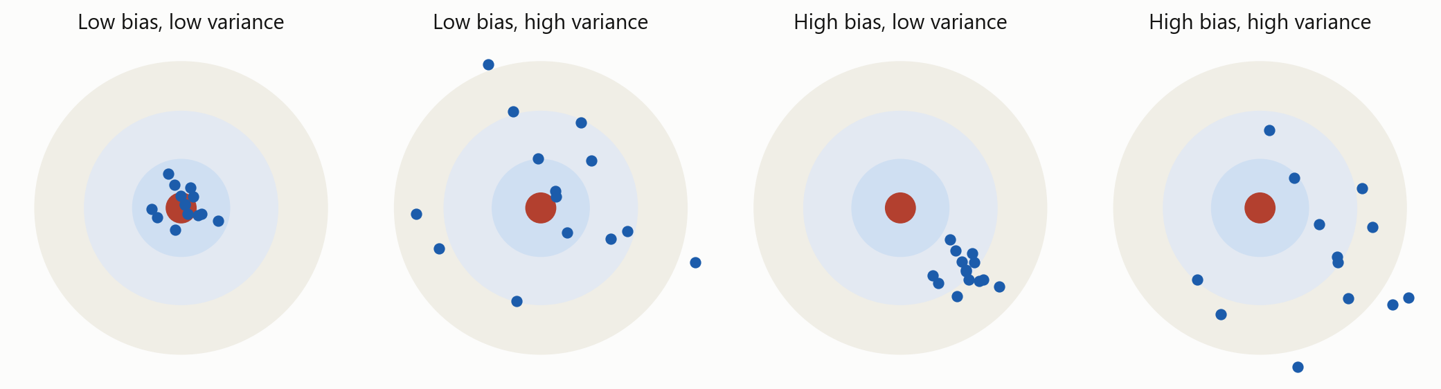
Both, on one target
Each dot is the model you would have got from one sample. Bias is how far the cluster sits from the centre. Variance is how spread out it is.
Three non-negative terms. Expected test error can never fall below the third one, and making one of the first two smaller usually makes the other larger.
This is a statement about expected error over all possible training samples, not about the one sample you happen to have.
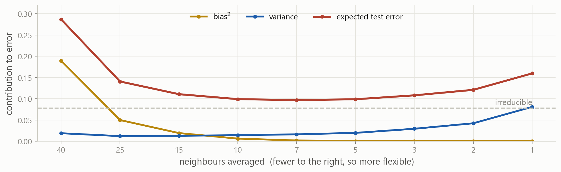
The trade-off, drawn
Bias falls, variance rises, and their sum has a minimum somewhere in between. The red curve is the same U as before, now explained.
The dial here is the number of neighbours rather than a polynomial degree, since it separates the two pieces more cleanly. Flexibility is the general idea; the particular knob does not matter.
What you actually do about it
Get more datavariance falls as n grows, and nothing else is as reliable
Use fewer featuresevery extra column is another way to fit noise
Simplify the modela linear model is hard to overfit, which is why it is still the benchmark
Penalise complexityridge and lasso deliberately add bias to remove more variance
Cross-validatereuse the training data to estimate test error, without touching the test set
Hold something backand do not look at it until you have finished deciding
The last three are the subject of the next block. You now know what problem they are solving.
There is no best model
There is no model that is best for every problem. Whether flexibility helps depends on the shape of the true f and on how much noise sits on top of it, and you do not get to see either one.
So the job is not to find the best model. It is to make the trade-off deliberately, and to be honest about how you measured it.
What stays with you
One table Rows are observations, columns are features, one column is the target.
Y = f(X) + \varepsilon You estimate f. You never remove \varepsilon.
Supervised or not A target column decides it. Number means regression, label means classification.
Cleaning is the work Missing, extreme, wrong scale, not numeric. In that order, most days.
Nothing from the future Not in a fill, not in a scaler, not in a split.
Pick the metric first MAE, RMSE and R² answer different questions. So do precision and recall.
Training error always falls Which is exactly why it cannot be used to choose a model.
Bias against variance Too simple misses the shape. Too flexible learns the noise.
Where this goes next
nowthe framework, the metrics, the trade-offno models fitted
nextmodel selection and cross-validationfinding the bottom of the U
thenregression and classification methods, trees, ensemblesscikit-learn
Everything from here is a different way of building \hat{f}. The questions you ask of it are the ones from today, and they do not change.
The course case, Part 4 case
Four sessions ago the case asked which of two stocks was riskier. It has grown every session since:
Part 1two stocks, a first look, arithmetic by hand
Part 2proper volatility, with loops and a function
Part 3all eleven stocks, pandas, and figures
Part 4the same data, reframed as a prediction problem
Case Part 4: this week
You will take the table you built in Part 3 and turn it into a learning problem:
choose a target, and build the features that are known before it
find the missing values and the extremes, and decide what to do about each
split by date, and say why the split has to be a date
choose the metric you would judge a model by, and defend the choice
state the prediction question precisely enough for somebody to answer it
You still do not fit anything. Part 4 finishes the setup, so that the first model you ever fit is one you already know how to judge.
Before the next session
Exercises: the statistical learning framework, data problems, metrics, and over- and underfitting. Longer than usual, and worth the time.
Case Part 4: the risk report becomes a prediction problem.
Stuck? Ask a friend, ask an AI for a hint rather than an answer, or email me at jobo@econ.au.dk.