Trees and forests
Machine Learning in Finance · Session 11
The models so far
| model | defined by | test score | |
|---|---|---|---|
| a number | linear regression (OLS) | \min_{\beta}\ \sum_i \big(y_i - \beta_0 - \sum_j \beta_j x_{ij}\big)^2 | RMSE 0.237 on one column, 0.248 on 19 |
| ridge | \min_{\beta}\ \text{RSS} + \alpha \sum_j \beta_j^2 | RMSE 0.218 | |
| lasso | \min_{\beta}\ \text{RSS} + \alpha \sum_j \lvert \beta_j \rvert | RMSE 0.217 | |
| a label | logistic regression | P(y = 1) = \sigma\big(\beta_0 + \sum_j \beta_j x_j\big) | AUC 0.748 |
| k-nearest neighbours | \hat p = \frac{1}{k} \sum_{k\ \text{nearest}} y_i | AUC 0.749, k = 25 |
Every model so far fits one formula to the whole table, or averages the nearest rows. Today’s model asks yes-or-no questions instead, with the cuts chosen from the data.
The volatility table
One row per trading day, and vol_next is the index’s volatility over the next 20 days. The split, the 19 columns and rmse are the ones ridge and lasso were scored with.
Today
- where a linear model stops on the volatility table
- a tree: questions, boxes and a formula
- growing a tree, one question at a time
- trees in scikit-learn, and drawing them with
plot_tree - how deep to grow a tree, and pruning
- bagging and random forests: many trees, averaged
- tuning a forest, what a search costs, and model size
- a tree for a label, on the credit table
The exercises and the case are where you practise each of these.
1 · Where a linear model stops
Part 1
A pattern in the volatility table that one coefficient per column cannot follow.
The error of linear regression, by level and direction
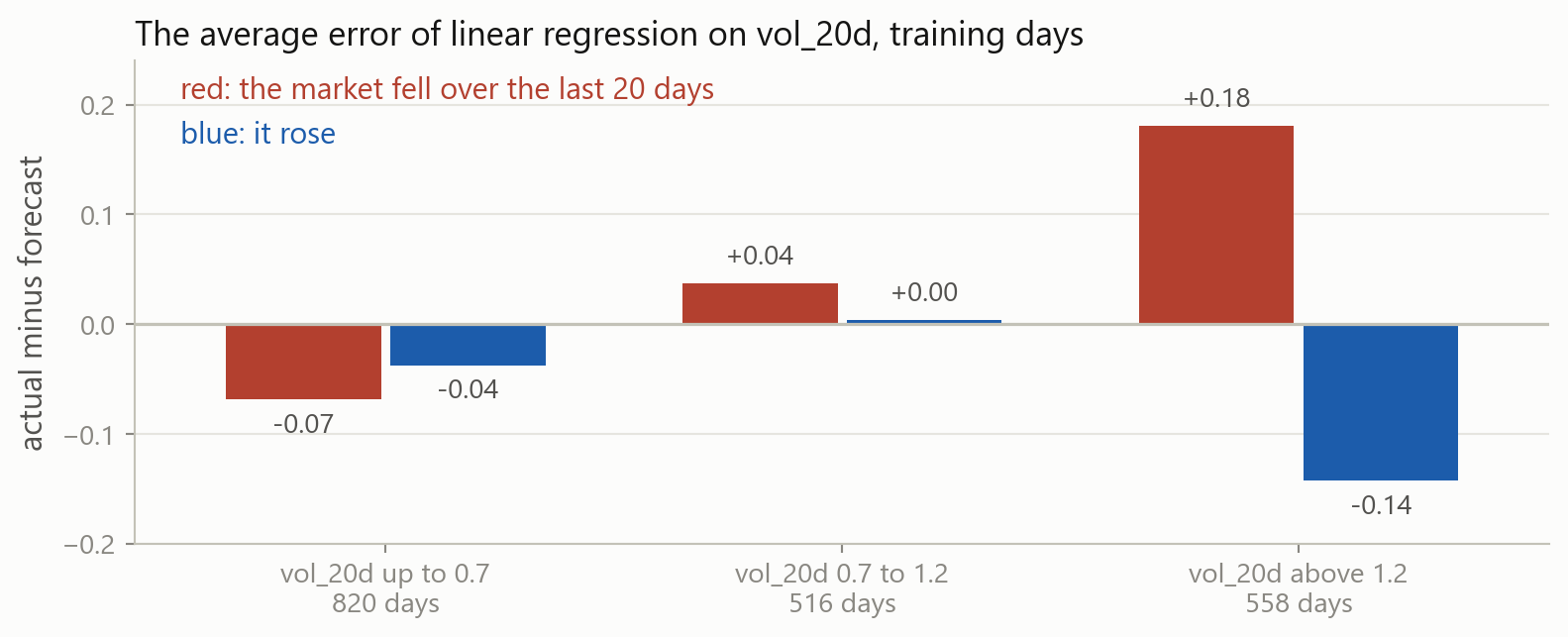
When vol_20d is above 1.2, linear regression is 0.18 too low after a 20-day fall and 0.14 too high after a rise. It gives both kinds of day the same forecast.
What a line can fit
What the table shows
When volatility is high, the next 20 days stay high after a fall and calm down after a rise. How much vol_20d matters depends on the market’s direction.
What a linear model can fit
One coefficient per column, the same after a fall and after a rise. A different slope for falls has to be written in by hand as a new column, at a cut already known.
A model of this table has to ask about the level first, and then about the direction when the level is high, with the cuts placed by the data.
2 · A tree of questions
Part 2
What a tree is, how it forecasts, and how to write it down.
A decision tree
A day answers the questions from the root down and lands in one leaf. A day with vol_20d at 1.5 and ret_20d at −0.6 gets 2.84: the average of 47 training days.
A tree on one column
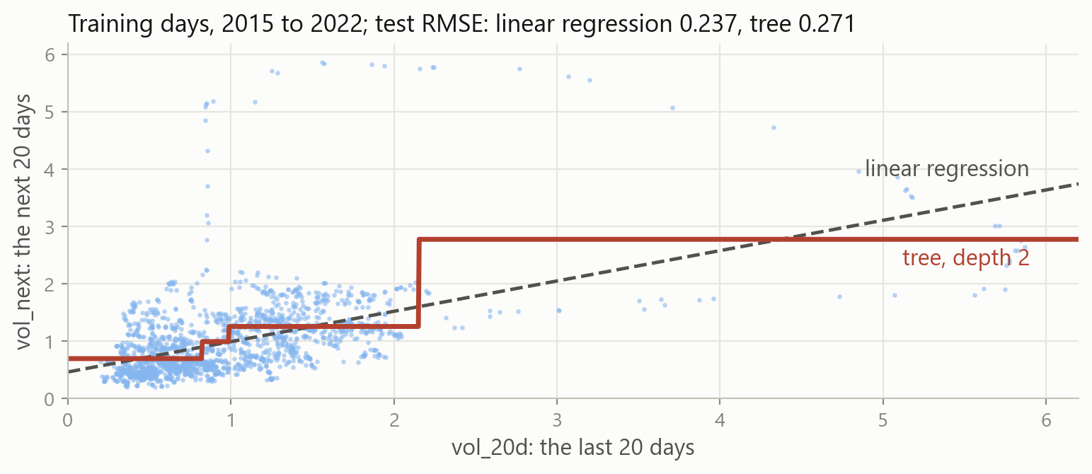
On vol_20d alone, a tree of depth 2 cuts at 0.82, 0.99 and 2.15 and forecasts four flat steps. On the test days it scores 0.271, linear regression 0.237.
The same tree as boxes
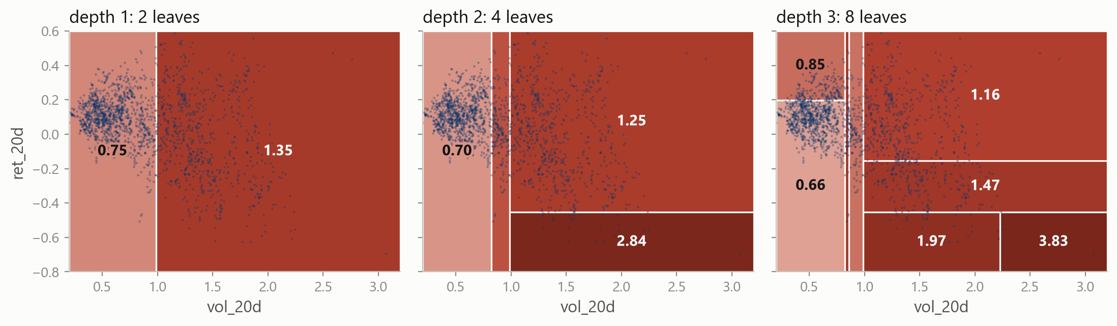
With two columns each question cuts the plane in two, and each level cuts every box again. Each box is shaded by its forecast; the dots are the training days.
A tree as a formula
\hat f(\mathbf{x}) = \sum_{m=1}^{M} c_m \,\mathbf{1}\{\mathbf{x} \in R_m\}
The leaves are boxes R_1, \dots, R_M, and c_m is the mean vol_next of the training days in box m. The indicator picks out the one box holding \mathbf{x}.
In the tree of depth 2, M = 4, and the four c_m are 0.70, 0.99, 2.84 and 1.25.
Three ways to forecast
| model | a forecast is | it needs |
|---|---|---|
| linear regression | one straight formula for the whole table | the shape written in: a column for every bend or interaction |
| k-nearest neighbours | the average of the k closest training rows | a scaler, and a distance that suits the columns |
| a tree | the average of the training rows in the same box | enough rows to place the cuts |
A tree forecasts from nearby training rows, as k-nearest neighbours does, but its neighbourhoods are boxes placed by the data, and a scaler changes nothing.
3 · Growing a tree
Part 3
How the questions are chosen, one at a time.
Six days
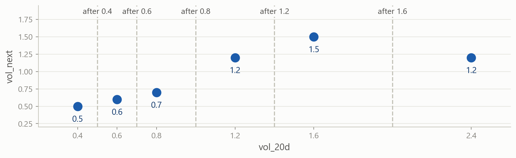
The six are real training days, rounded to one decimal. A question on vol_20d can cut them in five places; the best cut leaves each box with days as alike as possible.
The best number for one box
A box forecasts one number, c, for all its days. The squared error is smallest where its slope in c is zero:
\frac{d}{dc}\sum_{i} (y_i - c)^2 = -2\sum_{i} (y_i - c) = 0 \quad\Longrightarrow\quad c = \bar y
The best forecast is the box’s mean, and what is left is its RSS, \sum_i (y_i - \bar y)^2. Three days at 0.5, 0.6 and 0.7 forecast 0.6 and leave 0.02.
Every cut on the six
| cut after | left box | right box | total RSS |
|---|---|---|---|
| no cut | 6 days, mean 0.95: 0.815 | 0.815 | |
| 0.4 | 1 day, mean 0.5: 0 | 5 days, mean 1.04: 0.572 | 0.572 |
| 0.6 | 2 days, mean 0.55: 0.005 | 4 days, mean 1.15: 0.330 | 0.335 |
| 0.8 | 3 days, mean 0.6: 0.020 | 3 days, mean 1.3: 0.060 | 0.080 |
| 1.2 | 4 days, mean 0.75: 0.290 | 2 days, mean 1.35: 0.045 | 0.335 |
| 1.6 | 5 days, mean 0.9: 0.740 | 1 day, mean 1.2: 0 | 0.740 |
Each row adds up the RSS of the two boxes. The cut after 0.8 leaves 0.080, far below the rest: it separates the calm days from the busy ones.
The rule, in general
\min_{j,\;s}\;\Bigg[\sum_{i:\;x_{ij} \le s} \big(y_i - \bar y_{L}\big)^2 \;+\; \sum_{i:\;x_{ij} > s} \big(y_i - \bar y_{R}\big)^2\Bigg]
Column j and cut s make the two boxes, with means \bar y_L and \bar y_R. It is the RSS of least squares, with one constant per box in place of a line.
scikit-learn tries every column and every cut, and keeps the smallest.
The six, in code
rss adds up each value’s squared distance from the mean of its box. The cut after 0.8 leaves 0.02 on the left and 0.06 on the right, as in the table.
Every cut on vol_20d
A loop tries six cuts on the 1,894 training days. Without a cut the RSS is 908.5, and the cut at 1.25 leaves the least of these six, 752.1.
Recursive binary splitting, step by step
Each step keeps the cut with the smallest RSS inside one box, and earlier cuts are never revised: a greedy search. Three questions take the RSS from 908.5 to 617.6.
4 · Trees in scikit-learn
Part 4
Fitting a tree, drawing it with plot_tree, and reading its forecasts.
The best cut, found by scikit-learn
A stump, a tree with one question, tries every cut on both columns.
Reading one box
| line | in the top box | what it says |
|---|---|---|
| the question | vol_20d <= 0.986 |
True goes left, False right; vol_20d beat ret_20d |
squared_error |
0.48 | the box’s RSS divided by its days: the variance of vol_next |
samples |
1894 | the training days in the box |
value |
0.983 | the mean of vol_next in the box: its forecast |
The two leaves forecast 0.745 for the 1,154 calmer days and 1.353 for the 740 busier ones. Each leaf’s value is its c_m.
Your turn 1
Keep only the busy days, with vol_20d above 0.986, and fit a stump to them. Which question does it ask?
A mask keeps the rows where a condition holds, as in the loop over cuts. Fit on busy[pair] and busy["vol_next"].
Your turn 1: answer
Inside the busy box the best question is about ret_20d. After 20 days that fell 0.45 percent a day or more, the next 20 averaged 2.84; otherwise 1.25.
This is how a tree finds an interaction: each question is chosen for the rows of one box. A tree of depth 2 does it for every box.
A tree of depth 2
Each box of the stump gets a second question of its own. filled=True shades a box by its forecast, and impurity=False leaves out the error line.
Forecasts from the leaves
The 482 test days get only three different forecasts: none had high volatility after a steep fall. The error is 0.269, against 0.237 for linear regression.
A tree on all 19 columns
There is no scaler, because a cut compares one column with one number. Three levels of questions on all 19 columns score 0.390, worse than guessing the training average, 0.291.
Your turn 2
Draw tree in the clearer style. Which columns does it ask about, and why might that go wrong on the test days?
The column names are in columns. label="root" names the fields in the top box only, and precision=2 and fontsize=9 keep the text small.
Your turn 2: answer
The second question is Disney’s volatility above 1.26. It was on 330 of the 482 test days, so they got 1.20, while the index’s next 20 days averaged 0.80.
The first question sets aside the 27 most volatile training days, 26 of them in 2020: squared errors weigh the biggest misses most.
5 · How deep to grow
Part 5
A tree without a limit ends with a leaf for every training day.
The training days, scored predict
Grow a tree with no limit on vol_20d and ret_20d, and score it on the days it was grown on; the depth-2 tree scores 0.571 there. What will the error be?
A tree without a limit
The tree asks up to 32 questions and ends with 1,894 leaves, one for every training day. On the test days its error is 0.466, against 0.269 at depth 2.
Boxes around single days
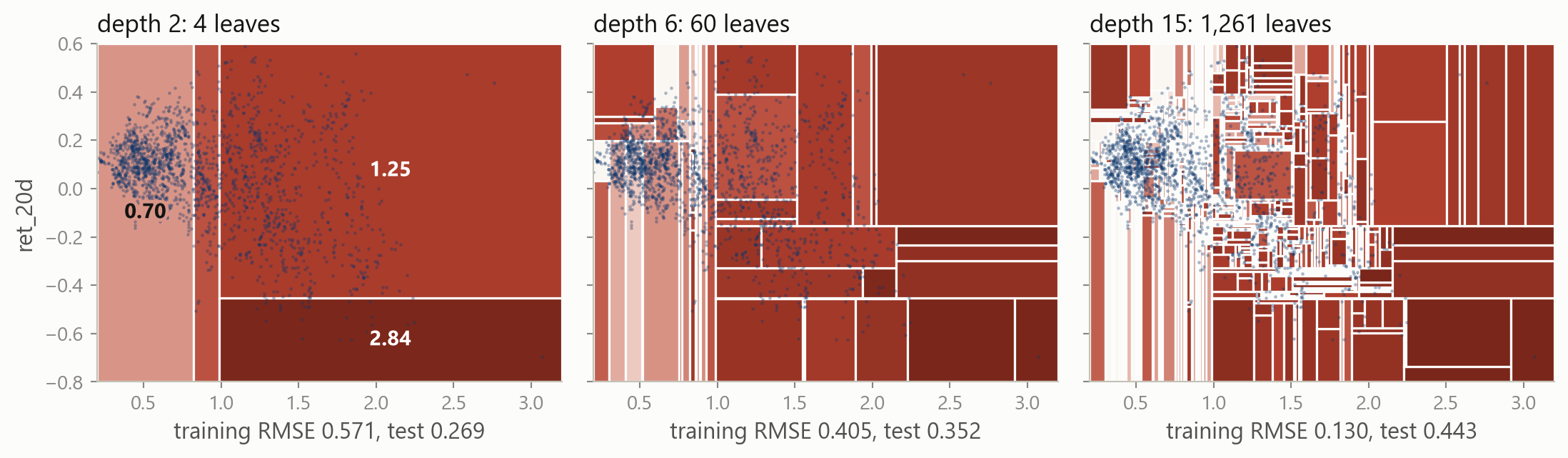
The same plane is cut at three depths. At depth 15 there are 1,261 boxes for 1,894 days: the training error is 0.130, the test error 0.443.
Depth against RMSE
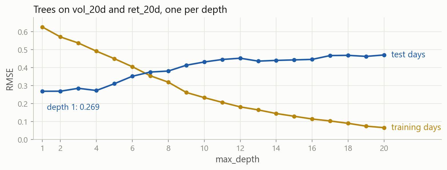
The test error is lowest at depth 1 or 2, 0.269, and climbs to 0.471 by depth 20. The training error falls towards 0.
Depth moves a tree along the bias-variance trade-off: a shallow tree is biased, and a deep one changes with every sample of days.
Depth on the folds
TimeSeriesSplit scores each fold on later days, as it did for ridge’s alpha; the folds include 2020, so their errors are larger. Depth 2 wins, at 0.637.
A minimum size for each leaf
A cut is allowed only if both boxes keep at least min_samples_leaf days. At 100 the folds’ error is 0.612, and the tree has 14 leaves and depth 6.
Pruning: a price for every leaf
R_\alpha(T) = R(T) + \alpha\,|T|
R(T) is the mean squared error left in the leaves of tree T, and |T| counts them; as in ridge, \alpha prices size. The folds choose 0.02: four leaves.
6 · Bagging and random forests
Part 6
Why one deep tree is not enough, and two ways of averaging many.
Two halves, two trees
Two full trees, each grown on a random half of the training days, differ by 0.39 on the average test day. The average of the two scores 0.329, better than either.
Why averaging helps
\operatorname{Var}\Big(\frac{1}{B}\sum_{b=1}^{B}\hat f^{\,b}(\mathbf{x})\Big) = \frac{\sigma^2}{B}
If B trees grown on independent samples each forecast with variance \sigma^2, their average has variance \sigma^2/B. There is one training set, so the samples come from it.
A deep tree has low bias and high variance, and variance is the part an average removes.
A bootstrap sample
replace=True puts each drawn day back, and nunique counts the distinct days. A day is missed by all n draws with probability (1 - 1/n)^n \approx e^{-1} = 0.37, so about 63 percent are in.
Bagging by hand
Each tree grows fully on its own bootstrap sample, and the average is \frac{1}{B}\sum_b \hat f^{\,b}(\mathbf{x}) with B = 20. This is bagging, from bootstrap aggregating: 0.320, where one full tree scored 0.410.
The first question of each bagged tree
BaggingRegressor grows and averages the trees and keeps them in estimators_. All 20 open with a volatility column, 11 with vol_5d.
Averaging trees that agree
\operatorname{Var}\Big(\frac{1}{B}\sum_{b=1}^{B}\hat f^{\,b}(\mathbf{x})\Big) = \rho\,\sigma^2 + \frac{1-\rho}{B}\,\sigma^2
\rho is the correlation between two trees’ forecasts. More trees shrink only the second term; the first stays until the trees are made less alike.
A random forest
max_features="sqrt" lets each question choose among 4 of the 19 columns, drawn at random. Without it the regressor uses every column, which is bagging.
The first questions in a forest
The 100 trees open with 12 different columns, and no column opens more than 22. Each tree is weaker, and the trees differ more.
The number of trees
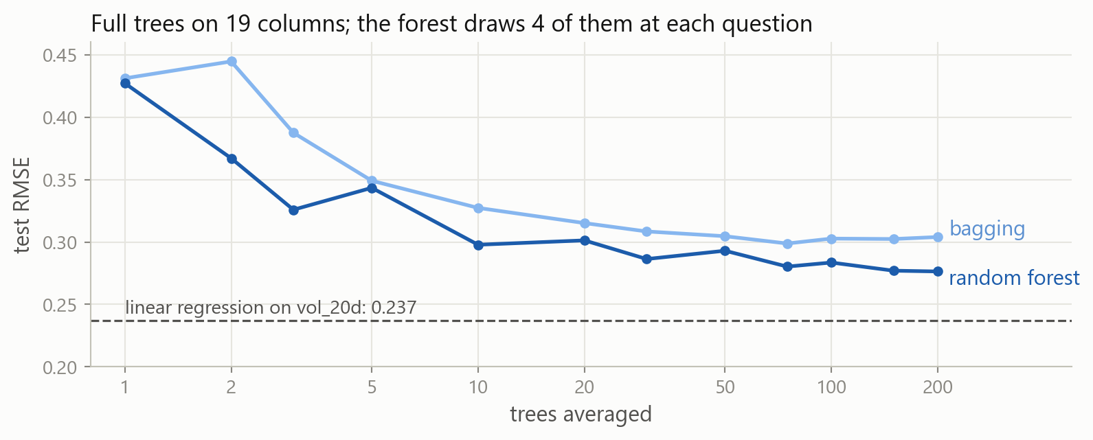
The forest’s average errs less than bagging’s at every size: 0.284 against 0.303 at 100 trees. Both flatten after about 50, above linear regression.
Out-of-bag rows on a time series
Each day is forecast by the trees whose sample left it out: an error of 0.252. On folds that score only later days it is 0.723, against 0.560 for ridge.
A day left out of a tree has its neighbours in the bag, and their next 20 days overlap its own by 19. On days, choose settings on TimeSeriesSplit folds.
Your turn 3
Build a forest like forest, but with leaves of at least 100 days, and print its test RMSE. Is it better than the forest of full trees?
min_samples_leaf sets the smallest leaf, as it did for one tree. Keep the other settings of forest.
Your turn 3: answer
Leaves of at least 100 days score 0.242, against 0.284 for full trees. Linear regression’s 0.237 is still lower.
7 · Tuning and its cost
Part 7
Why settings matter more for trees, what a search costs, and model size.
Settings to choose, model by model
| model | settings that change the fit | scikit-learn’s default | test RMSE, default and tuned |
|---|---|---|---|
| linear regression | none | 0.237 | |
| ridge | alpha |
1.0 | 0.248, then 0.218 |
| a tree, on two columns | max_depth, min_samples_leaf, ccp_alpha, and more |
no limit: one leaf per day | 0.466, then 0.241 |
| a random forest | the tree’s settings, plus n_estimators and max_features |
100 full trees on every column | 0.303, then 0.233 |
Ridge has one setting, and tuning it moved the error by 0.030. A forest’s defaults grow every tree down to single days, and tuning moved it by 0.070.
A grid over two forest settings
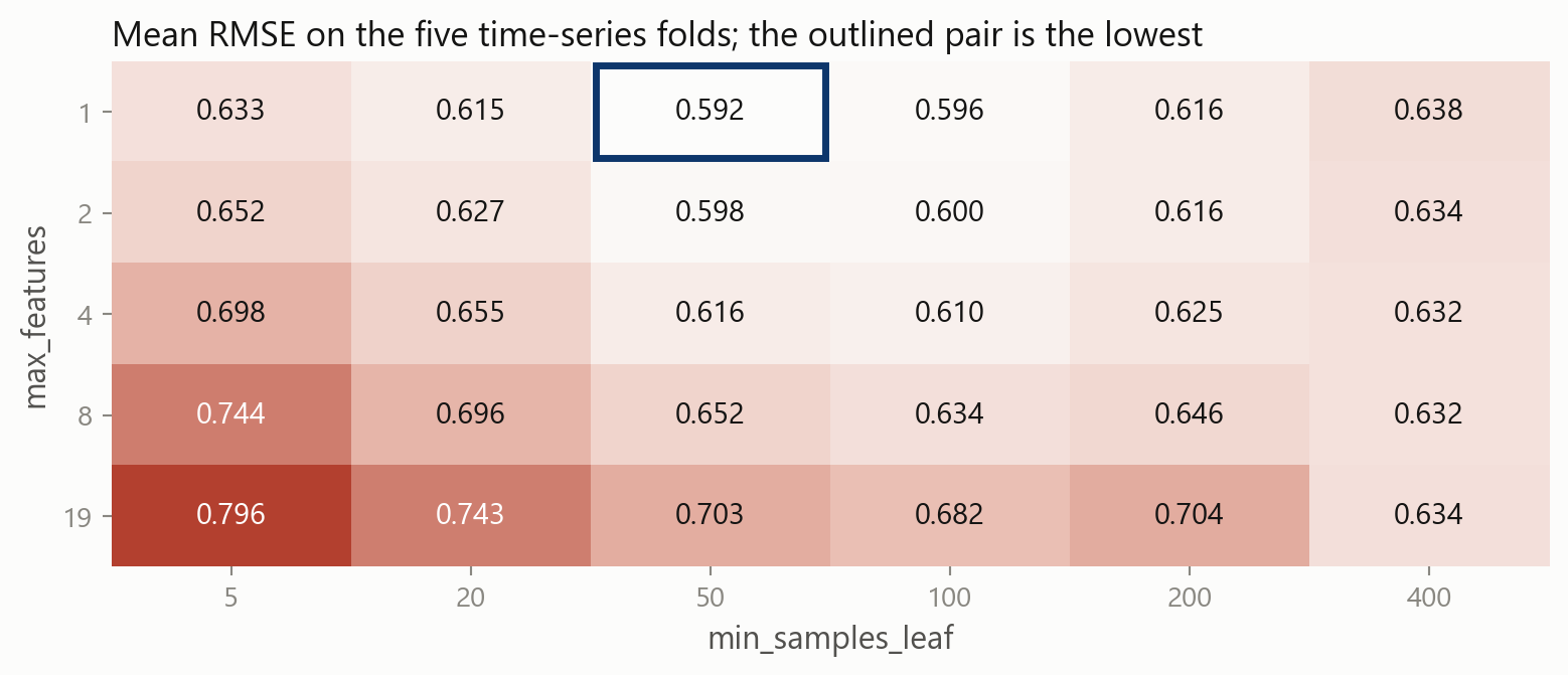
GridSearchCV scored 30 pairs on the five folds, 150 forests. One column per question and leaves of 50 days win: 0.233 on the test days, below linear regression’s 0.237.
What a search costs
| search, on five time-series folds | combinations | fitted | time on one core |
|---|---|---|---|
ridge: 7 values of alpha |
7 | 35 models | 0.1 s |
| a tree: 6 depths | 6 | 30 trees | 0.2 s |
a tree: 6 depths, 5 leaf sizes, 6 values of ccp_alpha |
180 | 900 trees | 5 s |
a forest: 5 max_features, 6 leaf sizes, 100 trees each |
30 | 150 forests, 15,000 trees | 26 s |
| the same, times 3 tree counts and 4 depths | 360 | 1,800 forests, 540,000 trees | 14 min |
Every setting multiplies the grid, and the folds multiply it again. The last search took 32 times as long and chose 100 trees of depth 3: 0.226 on the test days.
RandomizedSearchCV(model, grid, n_iter=20, ...) tries 20 combinations drawn at random, when the whole grid would take too long.
Timing one fit
time.perf_counter() reads a clock, so the difference is the seconds one forest took here. The grid of 30 pairs fits 150 forests; the last line is its minutes.
Model size against test error
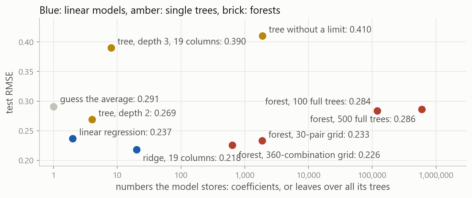
The largest model, 500 full trees with 598,735 leaves, took about 1,800 times longer to fit than ridge and forecasts worse than its 20 coefficients.
8 · A tree for a label
Part 8
The same questions on the credit table, with a share in each leaf.
The credit table
One row per card holder, and default is 1 for the 22 percent who defaulted the next month. On this split logistic regression scored an AUC of 0.748.
A classification tree
Each leaf’s value is the two shares; the second is the probability of default.
Gini, for labels
G = \sum_{k} \hat p_k\,(1 - \hat p_k)
For labels of 0 and 1, a box of n rows with k defaults has an RSS of k(n-k)/n. With two classes G = 2p(1-p), twice that per row, so the same cuts win.
DecisionTreeClassifier measures a box with Gini by default, and criterion="entropy" switches to D = -\sum_k \hat p_k \log \hat p_k.
A forest on the credit table
The rows are separate borrowers, so the out-of-bag score can be trusted: 0.781. On the test rows the forest scores 0.777, against 0.748 for logistic regression.
When to reach for a tree
The credit table
21,000 separate borrowers, a share of defaults that levels off, and a reversal that depends on another column. The forest beat logistic regression, 0.777 against 0.748.
The volatility table
1,894 days whose windows overlap, a relationship close to a straight line, and calm test years. Ridge beat every tree, 0.218 against 0.226 for the best-tuned forest.
Fit a linear model first, and make the tree beat it on folds that suit the rows.
When to change what
Always the size of each tree: max_depth or min_samples_leaf, on TimeSeriesSplit folds for days, or out-of-bag for a forest of separate rows. random_state, which fixes the samples and the order in which columns are tried.
Sometimes ccp_alpha, to prune a grown tree. n_estimators: more trees only cost time. max_features, the columns each question chooses among: "sqrt" makes a regressor a forest. class_weight, for labels. n_jobs=-1, to fit a forest’s trees on every core.
Rarely criterion, the error a cut is judged by. max_leaf_nodes, a cap on the number of leaves.
Never needed A scaler. A cut compares one column with one number, so StandardScaler in front of a tree gives the same forecasts.
What stays with you
Linear regression has one slope When volatility was high, linear regression on vol_20d was 0.18 too low after a fall and 0.14 too high after a rise.
A tree is questions, boxes and a formula \hat f(\mathbf{x}) = \sum_m c_m \mathbf{1}\{\mathbf{x} \in R_m\}: each leaf forecasts the mean of its training days.
Grown greedily, one cut at a time Every column and every cut, the smallest RSS, then again inside each box; a stump is one step. The best number for a box is its mean.
plot_tree shows it plot_tree(model, feature_names=...), with filled, impurity=False, precision and label="root". Each box shows its question, error, days and forecast.
Depth is the setting Without a limit: one leaf per training day, an error of 0 on them and 0.466 on the test days. Choose the size of a tree on TimeSeriesSplit folds.
Bagging and forests, for variance Averaging 20 bootstrap trees took the error from 0.410 to 0.320. Drawing columns at random makes the trees differ, and a tuned forest reached 0.226.
Tuning, cost and size Tuning moved the forest by 0.070 and ridge by 0.030. Each setting multiplies a grid, and 500 full trees forecast worse than ridge’s 20 coefficients.
A tree for a label The same cuts, judged by Gini. On the credit table the forest beat logistic regression; on the volatility table linear regression and ridge beat every tree.
Where this goes next
beforelinear regression, ridge and lasso for numbers; logistic regression and k-nearest neighbours for labelsformulas and neighbours
nowtrees, and forests that average them, for numbers and for labelsquestions, averaged
nextboosting: small trees grown one after another, each fitted to the errors so far, in scikit-learn, XGBoost and LightGBM; reading what a model has learned; the course as a wholethe wrap-up
Bagging and forests grow deep trees side by side and average away their variance. Boosting grows small trees in sequence, each correcting what the ones before it still get wrong, which removes bias.
Before the next session case
- Exercises: cuts scored by hand, stumps and trees drawn with
plot_tree, depth and pruning on the time-series folds, bootstrap samples, bagging and forests, grids counted and timed, and a tree for a label. - Case Part 11: the risk report’s volatility forecast gets a tree and a forest, held to its one-column model and to ridge on Apple and across the desk; a last question tries the forest on Part 9’s jump label.
Stuck? Ask a friend, ask an AI for a hint rather than an answer, or email jobo@econ.au.dk.