Boosting and reading a model
Machine Learning in Finance · Session 12
The models so far
| model | defined by | test score | |
|---|---|---|---|
| a number | linear regression | \min_{\beta}\ \sum_i \big(y_i - \beta_0 - \sum_j \beta_j x_{ij}\big)^2 | RMSE 0.237 on vol_20d |
| ridge | \min_{\beta}\ \text{RSS} + \alpha \sum_j \beta_j^2 | RMSE 0.218 | |
| lasso | \min_{\beta}\ \text{RSS} + \alpha \sum_j \lvert \beta_j \rvert | RMSE 0.217 | |
| a label | logistic regression | P(y = 1) = \sigma\big(\beta_0 + \sum_j \beta_j x_j\big) | AUC 0.748 |
| k-nearest neighbours | \hat p = \frac{1}{k} \sum_{k\ \text{nearest}} y_i | AUC 0.749 | |
| both | a tree | \hat f(\mathbf{x}) = \sum_m c_m \,\mathbf{1}\{\mathbf{x} \in R_m\} | RMSE 0.241, AUC 0.722 |
| a random forest | \hat f(\mathbf{x}) = \frac{1}{B}\sum_b \hat f^{\,b}(\mathbf{x}) | RMSE 0.226, AUC 0.777 |
A forest grows deep trees side by side and averages them. Today’s model grows small trees one after another, each fitted to what the ones before still get wrong.
The volatility table
The table and split that ridge and the forest were scored on: one row per trading day, 19 columns, and vol_next, the index’s volatility over the next 20 days.
Today
- what averaging cannot fix, and adding trees instead
- boosting: the definition, the procedure, and the procedure by hand
- how many trees, and stopping early
- XGBoost and LightGBM, the libraries used in practice
- boosting a label, on the credit table
- reading a model: which columns it uses
- the course’s models, side by side
The exercises and the case are where you practise each of these.
1 · What averaging cannot fix
Part 1
A forest removes the variance of deep trees. Small trees make a different error.
One stump, and 100 averaged
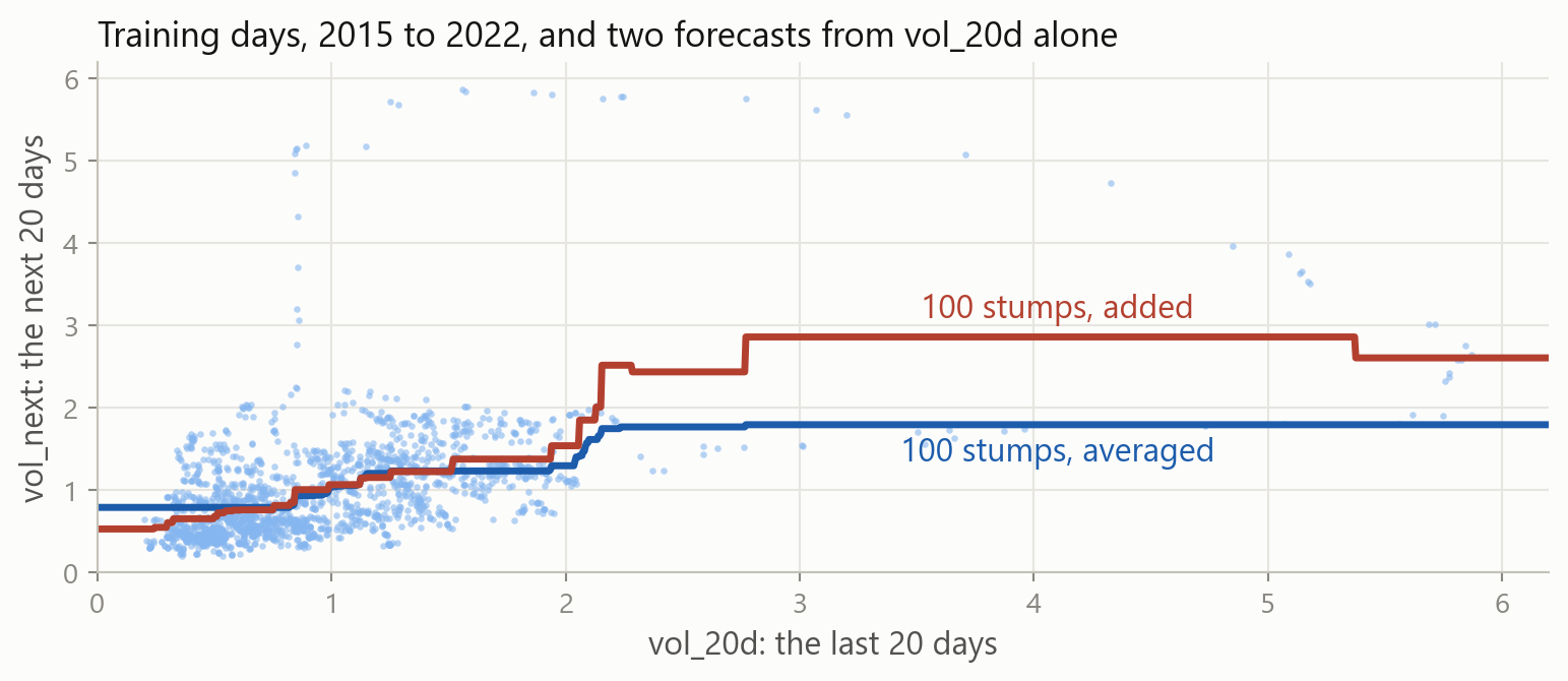
One stump errs 0.600 on the training days and 0.262 on the test days. The average of 100 stumps, each grown on a bootstrap sample, barely improves either.
Averaging stumps, and adding them
On vol_20d alone, 100 averaged stumps blur one step into a ramp from 0.79 to 1.80. Added one after another, 100 stumps build a staircase from 0.53 to 2.86.
Two ways to combine trees
Averaging: a forest
Deep trees, grown side by side on bootstrap samples, then averaged. Each tree fits its sample closely, so what the average removes is variance.
Adding: boosting
Small trees, grown one after another, each fitted to what the trees before it still get wrong. Each tree is too simple, so what the sum removes is bias.
An average of stumps is about as simple as one stump. A sum of stumps can bend wherever the data does.
2 · Boosting
Part 2
The definition, the procedure, and the procedure run by hand on six days.
Boosting as a formula
\hat f_M(\mathbf{x}) \;=\; \bar y \;+\; \nu \sum_{m=1}^{M} h_m(\mathbf{x})
Each h_m is a small tree and M is the number of trees; \nu, between 0 and 1, is the learning rate. The trees are added, so there is no 1/B.
Tree m is fitted to what the first m - 1 trees left: the residuals y_i - \hat f_{m-1}(\mathbf{x}_i).
The procedure
- Start every row at the mean: \hat f_0(\mathbf{x}) = \bar y.
- For each m = 1, \dots, M:
- compute the residuals on the training rows, r_i = y_i - \hat f_{m-1}(\mathbf{x}_i);
- fit a small tree h_m to the pairs (\mathbf{x}_i, r_i);
- add a step of it: \hat f_m(\mathbf{x}) = \hat f_{m-1}(\mathbf{x}) + \nu\, h_m(\mathbf{x}).
- Forecast new rows with \hat f_M.
Three settings shape the result: the number of trees M, the learning rate \nu, and the size of each tree.
Boosting the six days, step by step
The six days from last time, with \nu = 0.5: each step fits a stump to the dashed distances and adds half of it. Six stumps take the RSS from 0.815 to 0.038.
The six, in code
h is fitted to the residuals, not to vol_next, and half of its forecast is added on. The six RSS values are the diagram’s.
Your turn 1
Run the loop for 50 steps instead of 6. What happens to the RSS, and to the forecast?
The number of steps goes inside range. Compare the forecast with six["vol_next"].
Your turn 1: answer
The RSS falls to 0.0001, and every forecast is within 0.006 of its day: 50 stumps have learned the six days. On new days, that is overfitting.
Adding trees can always lower the training error, so the number of trees has to be chosen on other rows.
Residuals as a gradient
L_i = \tfrac{1}{2}\big(y_i - \hat f(\mathbf{x}_i)\big)^2 \quad\Longrightarrow\quad -\frac{\partial L_i}{\partial \hat f(\mathbf{x}_i)} = y_i - \hat f(\mathbf{x}_i)
The residual is the negative gradient of the squared error with respect to the forecast. Each tree is one step of gradient descent on the forecasts, hence the name gradient boosting.
With another loss, each tree is fitted to that loss’s negative gradient instead: for log-loss, y_i - \hat p_i.
Boosting by hand, on the table
100 stumps on the 19 columns, each fitted to what is left and added at \nu = 0.1. The test error is 0.222, where 100 averaged stumps scored 0.255.
Gradient boosting in scikit-learn
n_estimators is M, learning_rate is \nu, and max_depth=1 makes each tree a stump. The forecasts are the loop’s: 0.457 on the training days, 0.222 on the test days.
The forecast after 1, 10 and 100 stumps
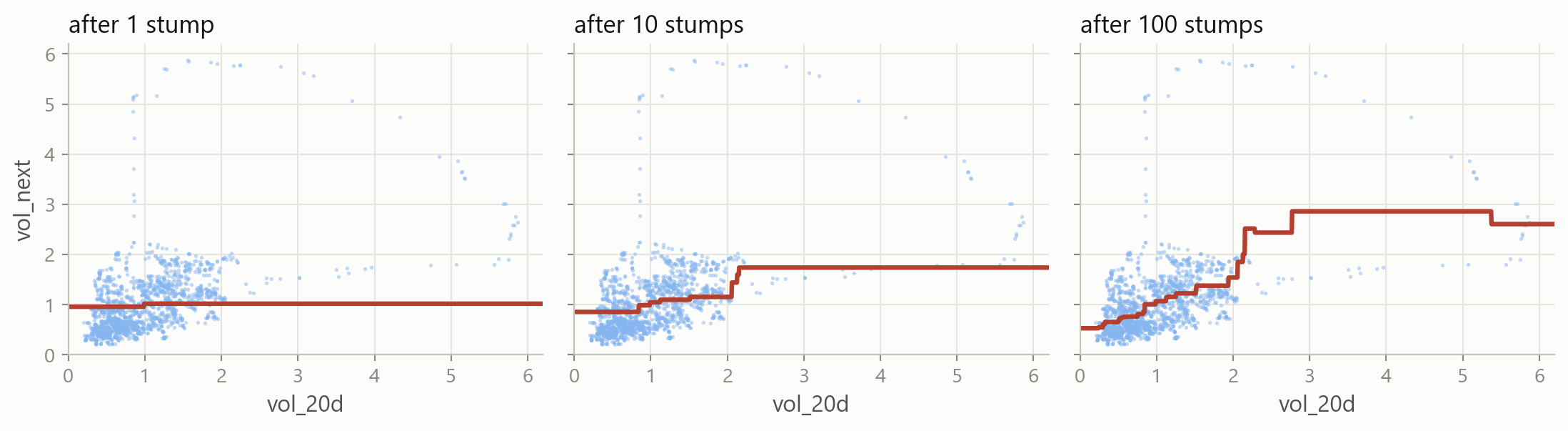
The first stump moves the forecast a tenth of the way: 0.96 to 1.02. After 10 stumps it spans 0.86 to 1.74, and after 100, 0.53 to 2.86.
3 · How many trees
Part 3
Every tree lowers the training error. On new days, too many trees do harm.
1,000 stumps predict
A forest’s test error only flattened as trees were added. Fit ten times as many stumps as boost: what will the test error do?
Test error against the number of trees
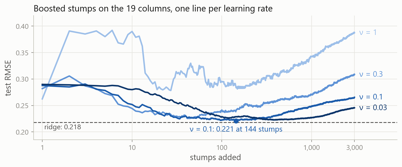
1,000 stumps err 0.350 on the training days and 0.248 on the test days. At every learning rate the test error falls, then rises; at 0.1 it is lowest near 144.
Your turn 2
Grow trees of depth 2 instead of stumps, with everything else as in boost. Better or worse on the test days?
max_depth sets the questions on each path, as for one tree. Stumps scored 0.457 and 0.222.
Your turn 2: answer
Trees of depth 2 fit the training days more closely, 0.299 against 0.457, and the test days worse, 0.269 against 0.222.
A tree of depth 2 can fit how two columns interact, and 100 of them also fit the noise in the training days.
The depth of each tree
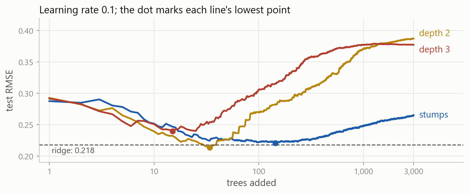
Deeper trees reach their lowest test error sooner and then climb faster: after 15 trees at depth 3, 34 at depth 2 and 144 with stumps.
Stopping early
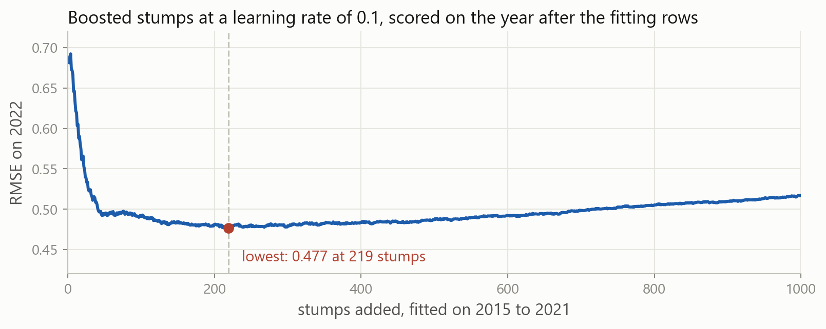
Fitted on 2015 to 2021 and scored on 2022 after every stump, the error is lowest at 219. That model scores 0.217 on the test days; ridge scored 0.218.
Early stopping on random days
n_iter_no_change=10 stops once 10 more trees have not helped on a random tenth of the training days: at 342 trees, with 0.226 on the test days.
A random day has its neighbours among the fitting rows, as out-of-bag days did, so the search stops late. On days, stop on a later block.
4 · XGBoost and LightGBM
Part 4
The two libraries most used for boosting in practice.
Two libraries built for boosting
XGBoost
Chen and Guestrin (2016). Bins each column, puts a penalty on every tree, handles missing values and uses every core. In 2015, 17 of the 29 winning solutions on Kaggle’s blog used it.
LightGBM
Ke and others, at Microsoft (2017). Bins each column and grows each tree leaf by leaf, to be fast on large tables. Both libraries follow scikit-learn’s pattern: create, fit, predict.
On 45 tables, tree-based models stayed ahead of deep learning on medium-sized data, about 10,000 rows (Grinsztajn, Oyallon and Varoquaux, 2022).
XGBoost in code
The same 100 stumps score 0.219, since XGBoost searches for cuts among 256 bins per column. Its defaults, 100 trees of depth 6 at a rate of 0.3, score 0.349.
A penalty on each tree
\sum_{i=1}^{n} L\big(y_i, \hat f(\mathbf{x}_i)\big) \;+\; \sum_{m=1}^{M} \Big(\gamma\, T_m + \tfrac{1}{2}\,\lambda \sum_{j=1}^{T_m} w_{mj}^2\Big)
T_m counts the leaves of tree m and w_{mj} are their values. reg_lambda is \lambda, a ridge penalty on the values; gamma is \gamma, a price per leaf, as in pruning.
The defaults are reg_lambda=1 and gamma=0: a light ridge penalty on the leaves, and no price for adding one.
LightGBM in code
LightGBM sizes a tree by its leaves, so num_leaves=2 makes a stump: 0.226. Its default of 31 leaves scores 0.346, and verbose=-1 silences its messages.
Depth by depth, or leaf by leaf
max_depth limits a tree grown depth by depth, and num_leaves one grown leaf by leaf. With the same leaves, a leaf-by-leaf tree goes deeper where the error is.
Early stopping in XGBoost
XGBoost scores every new tree on 2022 and stops 50 trees after the best. best_iteration counts from 0, so predict uses the first 244 stumps: 0.225.
Your turn 3
Suppose early stopping watched the test days instead of 2022. Pass them as eval_set: which score does it report, and is that a test score?
eval_set takes a list of (columns, target) pairs, as in xgb_stop. best_score is the lowest RMSE early stopping saw.
Your turn 3: answer
It keeps 30 stumps and reports 0.204, which would beat ridge’s 0.218. It is not a test score: the test days chose when to stop, out of 80 scores computed on them.
Rows that help choose a setting become validation rows. The test days report once, for a model chosen without them: here 0.225.
5 · Boosting a label
Part 5
The credit table, where trees beat logistic regression.
The credit table
One row per card holder; default is 1 for the 22 percent who defaulted the next month. On this split logistic regression scored 0.748 and the forest 0.777.
Boosting a label
\hat p_i = \sigma\big(\hat f(\mathbf{x}_i)\big), \qquad -\frac{\partial\, \text{log-loss}_i}{\partial \hat f(\mathbf{x}_i)} = y_i - \hat p_i
The trees are added on the log-odds scale, and each is fitted to y_i - \hat p_i, the gap between the label and the probability. The sigmoid turns the sum into a probability.
XGBoost on the credit table
100 trees of depth 3 at a learning rate of 0.1: an AUC of 0.777, the forest’s score, against 0.748 for logistic regression.
Four implementations of boosting
| model | how a cut is searched | fit, on one core | test AUC |
|---|---|---|---|
GradientBoostingClassifier |
every value of every column | 1.91 s | 0.776 |
HistGradientBoostingClassifier |
255 bins per column | 0.14 s | 0.776 |
XGBClassifier |
256 bins per column | 0.08 s | 0.777 |
LGBMClassifier |
255 bins, leaf by leaf | 0.08 s | 0.777 |
100 trees of depth 3, or of 8 leaves, at a learning rate of 0.1, on the 21,000 training rows. With bins, the same trees fit about 25 times faster.
Early stopping on separate borrowers
Borrowers are separate cases, so a random fifth of the training rows can decide when to stop: 91 trees of 15 leaves, and an AUC of 0.776.
When to change what
Always n_estimators, found by early stopping, with learning_rate: a smaller rate needs more trees. The size of each tree: max_depth, or num_leaves in LightGBM.
Sometimes subsample and colsample_bytree, a random share of the rows and columns for each tree, as in a forest; LightGBM also needs subsample_freq=1. The smallest leaf, min_child_weight or min_child_samples. reg_lambda.
Rarely gamma, a price per leaf. max_bin, the number of bins per column. objective, the loss that is boosted.
Never needed A scaler. A cut compares one column with one number, so scaling changes no forecast.
6 · Reading a model
Part 6
Which columns a model of many trees uses, measured two ways.
Importance from the cuts
XGBoost averages the fall in the loss over the cuts on each column and scales the results to sum to one. The two lateness columns take 87 percent.
A column of random numbers
LightGBM counts the cuts on each column. The noise gets the most, 582: each of its 21,000 values is a possible cut, where late_now has 9 values and gets 83.
What each library counts
| model | what feature_importances_ measures |
|---|---|
scikit-learn: trees, forests, GradientBoosting |
the fall in squared error or Gini from each column’s cuts, summed and scaled to one |
| XGBoost | the average fall in the loss per cut on the column, scaled to one |
| LightGBM | the number of cuts on the column; importance_type="gain" sums the fall instead |
scikit-learn: HistGradientBoosting |
it has no feature_importances_ |
All four measure on the training rows, where a flexible model has fitted noise too. LightGBM’s gain still gives the random column 8 percent, more than age.
Permutation importance
I_j = s - \frac{1}{K}\sum_{k=1}^{K} s_{k,j}
s is the model’s score on the test rows and s_{k,j} its score after the k-th shuffle of column j. Shuffling breaks the column’s link to the label and keeps its values.
It asks what the model loses without the column, on rows it did not fit.
Permutation importance in code
Shuffling months_late costs 0.112 of AUC, and shuffling the noise costs nothing. The column the cut counts ranked first comes last.
Two rankings of one model
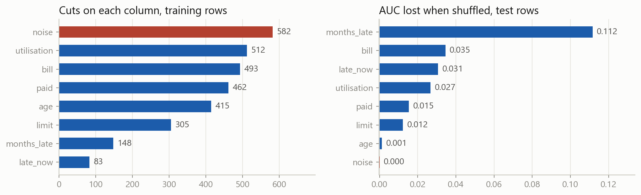
The noise is shown in brick. Counts of cuts reward columns with many possible cuts on the rows the model fitted; the shuffles are scored on the test rows.
Two correlated columns
| column | AUC lost when shuffled | AUC lost by a refit without it |
|---|---|---|
late_now |
0.031 | 0.012 |
months_late |
0.112 | 0.018 |
| both, together | 0.206 | 0.109 |
The two columns have a correlation of 0.72. A refit without either one loses little, because the other carries much of the same information.
Importance is what this model loses without a column, given the others. It is not the column’s effect on default.
7 · Choosing a model
Part 7
Every model of the course on both tables, what each is for, and the routine they share.
Both tables, every model
| model | volatility: test RMSE | credit: test AUC |
|---|---|---|
linear regression on vol_20d; logistic regression |
0.237 | 0.748 |
| ridge | 0.218 | |
| lasso | 0.217 | |
| k-nearest neighbours | 0.749 | |
| a tree | 0.241 | 0.722 |
| a random forest | 0.226 | 0.777 |
| boosted trees, stopped early | 0.217 and 0.225 | 0.777 and 0.776 |
On the volatility table, ridge, lasso and boosted stumps lie within 0.008 of each other. On the credit table, boosting and the forest tie, 0.029 above logistic regression.
The models of the course
| model | a forecast is | settings to choose | reach for it when |
|---|---|---|---|
| linear regression | a weighted sum of the columns | none | the relationship is close to straight, and always as a baseline |
| ridge, lasso | the same sum, with the weights shrunk | alpha |
there are many columns for the rows |
| logistic regression | a probability from a weighted sum | C |
the target is a label and the weights should be read |
| k-nearest neighbours | the average of the closest rows | n_neighbors |
there are few columns, all scaled |
| a tree | the mean of the box a row lands in | max_depth, min_samples_leaf |
the rules themselves are wanted |
| a random forest | the average of many deep trees | max_features, min_samples_leaf |
a strong model is needed with little tuning |
| boosted trees | the sum of many small trees | learning_rate, n_estimators, depth |
there are many rows, interactions and missing values |
All seven follow the same pattern in code: create, fit, predict, with the settings chosen on validation rows.
When to reach for boosting
Boosted trees first
Many rows, columns that bend or interact, missing values, a mix of types. On the credit table boosting and the forest reached an AUC of 0.777, logistic regression 0.748.
A linear model first
Few rows, a noisy target, a relationship close to a straight line. On the volatility table ridge scored 0.218, and boosting stopped early 0.217 and 0.225.
Fit a baseline and a linear model first. Keep a boosted model only if it wins on validation rows that suit the data.
The workflow, start to finish
- Load the table and look at it: shapes, types, missing values.
- Build the target and the features from the past only.
- Split by date, or at random when the rows are separate cases.
- Score a baseline: the average, or the majority class.
- Fit, and choose the settings on folds or on a later block.
- Open the test rows once, for the model you chose.
- Read the model: its coefficients, or its importance on the test rows.
- Report the score beside the baseline’s.
What you can now do
Sessions 1 to 3
Work with data
Load, clean, reshape and plot a table with pandas and matplotlib, using loops, functions and dictionaries.
Session 4
Frame a prediction
Build features and a target from the past only, split by date, and pick a metric and a baseline first.
Sessions 5 and 6
Fit and choose
Fit linear models, ridge and lasso, choose their settings on folds that suit the rows, and open the test rows once.
Sessions 8 and 9
Classify
Logistic regression and k-nearest neighbours; AUC, precision and recall, thresholds set from costs, and calibration.
Sessions 11 and 12
Grow trees
Trees, forests and boosted trees, tuned on the right rows, timed, and read through their importance.
Sessions 7 and 10
Run the whole workflow
From a raw table to a scored forecast, on house prices in Aarhus and on power prices in West Denmark.
What stays with you
Averaging cannot remove bias 100 averaged stumps err 0.577 on the training days, against 0.600 for one. 100 stumps added one after another err 0.457.
Boosting fits what is left \hat f_m = \hat f_{m-1} + \nu\, h_m: each small tree h_m is fitted to the residuals, the negative gradient of the loss.
More trees can overfit At \nu = 0.1 the test error is lowest near 144 stumps, 0.221, and 0.265 at 3,000. Deeper trees turn up sooner.
Stop on a later block XGBoost stopped on 2022 at 244 stumps: 0.225. Stopped on the test days, it reported 0.204, a score those days chose.
XGBoost and LightGBM Bins, a penalty on each tree, growth leaf by leaf: on the credit table the same trees fit about 25 times faster than in GradientBoosting.
Boosting a label Each tree is fitted to y_i - \hat p_i on the log-odds scale. On the credit table, 0.777: level with the forest.
Importance, two ways Counts of cuts ranked a column of random numbers first. Shuffles on the test rows ranked it last, at zero.
Correlated columns share importance Shuffled together, late_now and months_late cost 0.206 of AUC; a refit without either one loses under 0.02.
Where this goes next
beforePython and pandas; linear regression, ridge and lasso; logistic regression and k-nearest neighbours; trees and forestsSessions 1 to 11
nowboosting, XGBoost and LightGBM, and reading a modeltrees, added
nexta final case lecture, and the wrap-up of the courseto finish
Every model came with the same routine: a baseline to beat, settings chosen on rows that suit the data, and a test set opened once.
After this session case
- Exercises: the six days boosted by hand, the gradient behind the residuals, the number of trees chosen on 2022 and on the folds, XGBoost and LightGBM, importance measured four ways, and a target with nothing in it.
- Case Part 12, the last part: boosting for the risk report’s forecast and warning, then every model fitted since Part 4 side by side, and the report as it would go out.
Stuck? Ask a friend, ask an AI for a hint rather than an answer, or email jobo@econ.au.dk.